Hydrologic Response in an Urban Watershed as Affected by Climate and Land-Use Change


1
Department of Agricultural & Biological Engineering, Purdue University, West Lafayette, IN 47906, USA
2
Geology Department, Faculty of Science, Suez Canal University, Ismailia 41511, Egypt
*
Author to whom correspondence should be addressed.
Water 2019, 11(8), 1603; https://doi.org/10.3390/w11081603
Submission received: 10 July 2019
/
Revised: 27 July 2019
/
Accepted: 31 July 2019
/
Published: 2 August 2019
(This article belongs to the Special Issue Urban Water Accounting)
Abstract
:The change in both streamflow and baseflow in urban catchments has received significant attention in recent decades as a result of their drastic variability. In this research, effects of climate variation and dynamics of land use are measured separately and in combination with streamflow and baseflow in the Little Eagle Creek (LEC) watershed (Indianapolis, Indiana). These effects are examined using land-use maps, statistical tests, and hydrological modeling. Transition matrix analysis was used to investigate the change in land use between 1992 and 2011. Temporal trends and changes in meteorological data were evaluated from 1980–2017 using the Mann–Kendall test. Changes in streamflow and baseflow were assessed using the Soil and Water Assessment Tool (SWAT) hydrological model using multiple scenarios that varied in land use and climate change. Evaluation of the model outputs showed streamflow and baseflow in LEC are well represented using SWAT. During 1992–2011, roughly 30% of the watershed experienced change, typically cultivated agricultural areas became urbanized. Baseflow is significantly affected by the observed urbanization; however, the combination of land and climate variability has a larger effect on the baseflow in LEC. Generally, the variability in the baseflow and streamflow appears to be heavily driven by the response to climate change in comparison to variability due to altered land use. The results reported herein expand the current understanding of variation in hydrological components, and provide useful information for management planning regarding water resources, as well as water and soil conservation in urban watersheds in Indiana and beyond.
1. Introduction
Water is an indispensable natural resource for life and an increasingly limiting factor to socioeconomic developments [1]. Water resources issues are widely discussed throughout the world. Addressing these issues requires information about the factors that drive hydrological changes and their related effects on local water resources. Evaluating water resources becomes a complex task that needs to consider many facets. Studies that detail the spatial and temporal distribution of water resources are of vital significance to inform management strategies.
Both climate variation and human actions act as stressors that contribute to putting water resources under severe pressure [2]. Intensive human activities apart from climate change, such as land-use change, urbanization, economic development and population growth, have posed unprecedented impacts on watershed hydrological conditions. For example, these stressors can alter surface runoff, evapotranspiration, baseflow, the frequency of floods, annual mean discharge, flow routing time, peak flows and volume [3]. Moreover, the pressures of these human activities are associated with climate variation which in turn will affect water sustainability for socioeconomic developments [4].
The impacts of individual factors on watershed hydrology theoretically cannot be separated [5]. This coupling effect, together with water withdrawal and retention, contributes to the uncertainties in identifying the specific impact of each factor on watershed hydrology [6]. This creates difficulty in inferring causation on a sufficient scale, and therefore it remains unclear which of these factors dominantly contributes to watershed hydrology [4,5]. Indeed, several reports show conflicting conclusions when the combined hydrological responses are measured [6,7,8,9]. Climate variation exerts a control on dominant agricultural and land use practices including their spatial properties [10,11,12]. The joint impact on hydrology of climate variation and land use change has been shown to be similar to that of a single climate change factor [13,14]. Hence, identifying the distinct impacts of changing land use from climate variability and understanding the water balance is considered a particular challenge for studies on operational management of reservoirs and river basins.
In recent years, several investigators have studied the effect of climate variation and land use change on watershed hydrology [15,16,17]. Zhang et al. [16] studied these effects on streamflow in the China Fenhe River Basin. The study found a stronger influence of land use on streamflow than climate change. Xu et al. [17] similarly showed that land use affects streamflow variation twice as much across more than 50 watersheds throughout the Midwestern United States.
Although an increase in high streamflow and decrease in low streamflow is often associated with urbanization [18], the impact of land use change often varies with climate [14]. On the other hand, the changes in watershed hydrology and annual water balance can also be attributed to climate variability, especially in large scale watersheds, likely caused by compensatory effects in a complex watershed [19]. Novotny and Stefan [20] reported a correlation between the mean annual streamflow trend and rainfall in five major Minnesota River watersheds, while in Indiana rainfall has shown a strong relationship with low flow [21]. In addition, Frans et al. [22] concluded that wet climates, rather than land use change, had the most impact on streamflow in the Upper Mississippi River Basin. Comparable research was conducted by Tan et al. [23] in the Johor River Basin in Malaysia; results indicated that climate change was the main driving force that impacted watershed hydrology. In the Yellow River Basin in China, climate fluctuation accounted for a 10 mm per year reduction in mean annual streamflow [24]. River discharge significantly increased in the upper Syr Darya river basin due to temperature increase from 1930 to 2006 [25]. Duan et al. [26] evaluated the effects of projected climate change scenarios on watershed streamflow in the Upper Ishikari river basin in Japan, finding annual mean streamflow will likely increase for future climate scenarios. Therefore, it is important to distinguish between effects related to land-use changes and those due to climate variability for accurate estimation of surface and groundwater responses.
Impacts of these factors on watershed hydrology is different across watersheds. Therefore, sites must be evaluated on a local scale [27]. Due to limited available data, it is essential to use both comprehensive and physical tools to extract as much information about hydrologic responses as possible [28]. Hydrological models are considered an appealing approach to carry out impact assessment studies, as they provide a conceptualized framework to be used in scenario studies on the relationship between hydrological components, land-use change and climate variability [29]. Model parameters can have physical meaning as related to measurable landscape properties and meteorological conditions [30], and explicitly represent spatial variability [31]. Initial model parameters describing vegetation, land use and soil types are called physically based parameter values; they can be adjusted to improve streamflow simulation through subsequent model calibration processes [32].
Recently, water resource managers and modelers have counted on hydrological models to identify alternative strategies for water resource allocation and to obtain more information about watershed systems, hydrological processes, and their responses to both anthropogenic and natural factors [33], including insight regarding the impacts of future climate projections [34]. Some of these models incorporate the watershed’s heterogeneity and the spatial distribution of land use, topography, soil type, and meteorological conditions [35]. Among these models is the Soil and Water Assessment Tool (SWAT) model. SWAT is a conceptual mathematical semi-physical, semi-distributed based model [36]. SWAT employs parameters with time steps at a daily scale [37]. The model is designed with basic components, for example, climate, sediment type, nutrients, and hydrology [38]. This allows for interconnections of different physical processes that occur in the environment, making it the model able to evaluate how the hydrological components are impacted by land management methods in complex catchments with different land covers, and climate scenarios in extreme events such as droughts and floods [39].
Streamflow and baseflow in watersheds in the US Midwest region reported upward trends with both urbanization and climate change [16,32]. While previous streamflow and baseflow trend investigations included urbanized watersheds in the Midwest region [40], they lacked integration analysis, which exclusively focuses on the interactive impacts of land and climate variability on urbanized catchments. In addition, multiple factors, nonlinear relationships, and poor understanding of mechanisms limits the ability to attribute causation [41]. Therefore, the current study focuses on this issue through a systematic investigation, taking into account the effects of both individual and coupled impacts of human and natural impacts.
The study area, Little Eagle Creek (LEC) in central Indiana is an ideal candidate site for this type of study because it has been previously examined for many of water-related issues and has substantial data available for this study. Previously, the LEC was investigated to evaluate impacts of urbanization on water issues. Bhaduri et al. [42] utilized the Long-Term Hydrologic Impact Assessment (L-THIA) model with different land use patterns to evaluate nonpoint source (NPS) pollution and to assess impacts on annual average runoff from the watershed. The study concluded that the 18% increase in urban areas, from 1973 to 1991, resulted in an estimated 80% and 50% increase in annual average runoff and pollutant loads, respectively. Grove et al. [43] conducted a similar study; results were consistent with Bhaduri et al. [42], though they reported an increase of 60% in average annual runoff depth from 1973 to 1991 due to urbanization. Doyle et al. [44] reported that stream incision occurring in the LEC was a response to urbanization though the measures of channel stability were not directly related to levels of urbanization. Choi et al. [45] estimated an increase in direct runoff from 49% to 63% during a 12-year time-span (1973 to 1984), suggesting that urbanization impacted direct runoff more than total runoff. In addition, they also pointed out that substantial baseflow is essential to maintain sound stream ecosystems in the LEC watershed. In their attempt to minimize the runoff impact of urbanization in the LEC, Tang et al. [46] were able to reduce runoff increase by as much as 4.9% from 1973 to 1997.
More recently, Lim et al. [47] estimated the effect of initial abstraction and urban growth on estimated runoff using modified curve number values in the L-THIA model. Results showed improvements in the prediction of direct runoff over the long term, resulting from using modified curve numbers and hydrologic soil groups for urbanized areas. Lim et al. [48] reported that improved input parameters could improve L-THIA model performance.
The overall aim of this research was to evaluate the response of watershed streamflow and baseflow to climate variability and land-use change in an urban watershed in Indiana, based on simulation following a comprehensive calibration. The specific objectives are: (A) to evaluate long-term trends of historical streamflow, land use and rainfall in an urban watershed; (B) identify changes in land use from 1992 and 2011 through transition matrix analysis; (C) calibrate and validate SWAT model performance, using different land-use patterns for different periods; (D) investigate hydrological streamflow and baseflow sensitivity to land-use change and climate variability; and (E) simulate the joint effects of both climate and land-use change on hydrology in this watershed. For this goal, plausible scenarios of land-use change and climate variation were developed based on trends and information exploited from the Little Eagle Creek (LEC) watershed. The results obtained provide useful information towards the improvement of the current understanding of hydrological component variation. Additionally, the results are informative to planning and management strategies for water resources that seek to minimize the undesirable effects of land-use change and climate variation as well as water and soil preservation in urban watersheds in Midwestern USA and potentially beyond.
2. Materials and Methods
2.1. Study Area
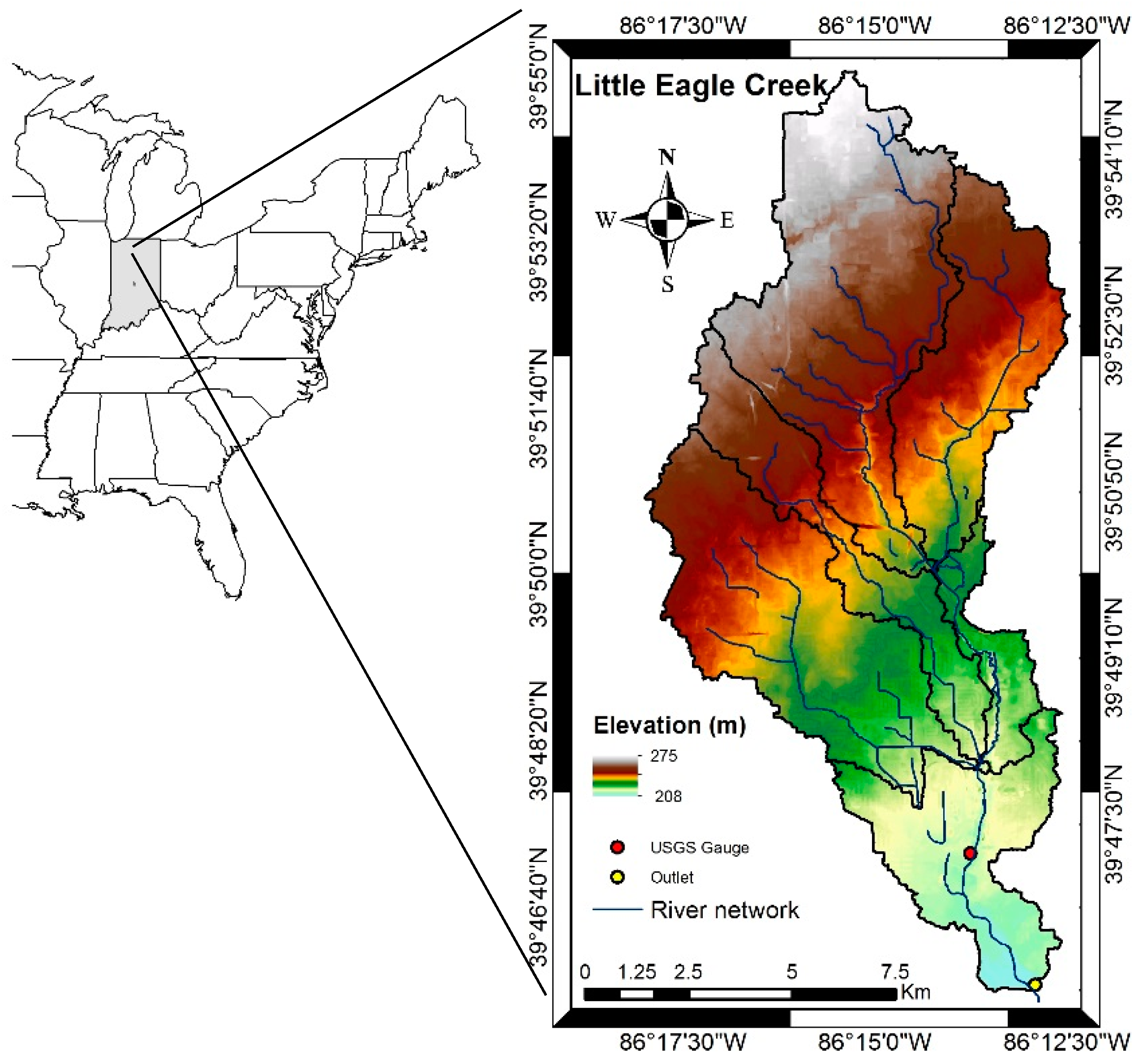
Little Eagle Creek (LEC) Watershed is located in northwest Indianapolis, Marion County in central Indiana (Figure 1). The watershed covers approximately 74.5 km2 (USGS Gauge 03353600), with annual precipitation ranging from 795 to 1443 mm from 1980 to 2017. The minimum, maximum and mean elevation in the area were 208, 275 and 242 m above sea level, respectively. This watershed has undergone significant urbanization in recent decades due to its proximity to the capitol city, creating a possible threat to the watershed’s water resources. Current land use includes 95.8% typical urban residential and commercial categories that are the majority of land use, 3.2% non-urban natural grass and forest, and only 0.5% agricultural and cultivated areas [48]. Regionally, thunderstorms occur throughout the year and particularly in the spring and summer seasons [44].
2.2. Datasets Description
The explicit datasets used to build and calibrate the SWAT model can be classified into statistical, geographical or spatial data for hydrologic simulation. The statistical data includes hydro-meteorological data, while the spatial data include Digital Elevation Model (DEM), land use and soil maps.
2.2.1. Hydro-Meteorological Data
The sets of data used herein includes long-term daily meteorological data from 1980–2017, (precipitation, minimum/maximum air temperature, wind speed, solar radiation and humidity), obtained from the National Climate Data Center (NCDC) (see Supplementary Materials). The weather station was approximately 2.5 miles from the LEC watershed. Hydrological streamflow data were based on observations from 1980 to 2017 at a gauged station within the watershed. The streamflow data were used for the calibration and validation of the SWAT model and to separate the baseflow from the direct discharge. Streamflow data were complete with no missing records (see Supplementary Materials).
2.2.2. Topography and Soil Type
The results reported herein used elevation, flow direction, accumulation, stream network, channel properties, slope and aspect to describe the topography of the study areas. The DEM topographical data used had a resolution of 10 m by 10 m and was obtained from the Geospatial Data Gateway (GDG). DEM data were first used to delineate watersheds into sub-basins and the drainage patterns and identify flow direction of the land surface terrain. Soil type, slope and land use was then used to classify these sub-basins into small Hydrologic Response Units (HRUs) [49]. HRUs demonstrate the smallest representative unit of the watershed. Soil type data were obtained from Soil Survey Geographic Data (SSURGO) with a resolution ranging from 1:12,000 to 1:63,630. The SWAT model requires these soil parameters, as the soil’s chemical and physical properties play an important role in evaluating water movement within the HRU [50].
2.2.3. Land-Use Data
This study used digital land-use data acquired from the National Map Viewer (NMV). To examine the consequence of land-use change on the hydrology of the watershed, raster land-use maps of 1992 and 2011 were used in this research.
2.2.4. Hydrological SWAT Model
The SWAT model, developed by the USDA Agriculture Research Service, is designed to model hydrology at the scale of a watershed [36]. The SWAT model is structured on fundamental components of action, such as: Climate, hydrology, sediment, nutrients and management [51,52,53] and can be used to predict the variation in these components by change in land use and climate. SWAT follows a defined operating sequence; (1) data preparation, (2) discretization of sub-basins and definition of HRUs, (3) sensitivity analysis, (4) parameter calibration and (5) validation. The computational simulations in this study were performed with the SWAT 2012 extension, using the ArcSWAT interface of ArcGIS 10.4.1 [37].
The hydrologic routine within SWAT includes the vadose zone processes (plant uptake, evaporation, infiltration, lateral flows, and percolation), groundwater flows and snow fall and melt. The hydrologic cycle in the SWAT model is based on water balance and is expressed as follows [54]:
where is the final soil water content (mm); is the previous soil water (mm); t is the time step (day); , and are the precipitation, surface runoff, and evaporation measurements on day i (mm), respectively; is the amount of water entering the vadose zone from the soil profile on day i (mm), and is the amount of return flow on day i (mm).
For each HRU, SWAT simulates surface water and shallow groundwater. Then, these values are calculated for the sub-basins by a weighted value using the combined HRUs. Using daily rainfall amounts and a modified version of the Soil Conservation Service (SCS) curve number method, surface runoff is computed. Estimation of baseflow and groundwater flow is based on the hydraulic conductivity of the shallow aquifer, water table height and the distance between the sub-basin and main channel.
The SWAT framework serves to conceptualize the relationship between climate variation, land-use change and human activities and their synchronous impacts on watershed hydrology [8]. For further information on the SWAT model, refer to the online resource at https://swat.tamu.edu/ and Arnold et al. [37].
2.3. Methods
2.3.1. Land-Use Change Detection
Post-classification change detection analysis was applied to determine the temporal change in land use of the watershed. Statistics for change detection from the land-use maps have been obtained over time (1992 and 2011) for this research through the thematic overlay of the classified land-use maps using pixel-by-pixel cross-tabulation analysis. This was used to evaluate the “from-to” change detection matrix table that shows the major gains and losses in each category [55,56,57].
2.3.2. Temporal Trend Analysis Method
The modified Mann–Kendall (M-K) test suggested by Hamed and Rao [58] was applied in this study to analyze the change in annual precipitation and temperature in the LEC watershed. The M-K test is a widely-used, non-parametric, rank-based test [59], that has found considerable use in hydrology and climatology given its robustness and ability to avoid the effects of extreme values [60]. The modified M-K was chosen for this research due to the presence of negative and positive serial correlations recognized in meteorological data, that can result in overestimation or underestimation of the trends [3]. The M-K test can identify the magnitude of the slope of individual variables, whereby a positive slope magnitude indicates an upward trend and vice versa [61,62]. The M-K test statistic is calculated by:
and
where S is the M-K test statistic, xj and xi are the sequential data values; and n is the dataset size [62].
2.3.3. Baseflow Separation Using Web-Based BFlow
Baseflow separation methods were used for streamflow separation into direct runoff and baseflow since the measurement of baseflow is considered more difficult as compared to streamflow measurement. Baseflow measurements were calculated from USGS daily streamflow data using the ‘BFlow’ digital filter program. The BFlow program calculates baseflow by filtering streamflow data three times (1-Pass, 2-Pass and 3-Pass) through the filter in Equation (6), allowing the user to select the required number of passes for baseflow evaluation [63,64].
where is the baseflow, is the filter parameter (0.925), is the total streamflow, and t is the time step. Equation (1) is applied only when BF ≤ Qt [65].
2.3.4. Scenario Analysis: Modeling Hydrological Response to Climate Variability and Land-Use Dynamic
Land-use data and HRU outputs for the LEC watershed showed a dramatic change in impervious cover after 1992. However, little change was detected in impervious cover between 2001 and 2011, as the watershed area was mostly urbanized by 2001. Therefore, at this stage, only land-use data for 1992 and 2011 were considered in the calibration and validation processes for the two climate periods. Land-use data from National Land Cover Database (NLCD) for 2001 and 2006 were not used in further analysis.
To evaluate the separate and combined influences of land-use dynamics and climate alteration on hydrological components, the “fix-changing” approach was used, in which one factor at a time was changed while holding others constant. Based on the change detection analysis of temporal trends of precipitation and temperature and land-use change, the meteorological data from 1980–2017 were divided into two periods, with each period including one land use map. The period of 1980–1998 was called CP1, representing the 1980s and 1990s and was considered the baseline period, and the impacted period of 1999–2017 was called CP2 and represented the 2000s and 2010s. The 1992 land-use map for 1992 represented the patterns in CP1, while the 2011 land-use map for 2011 was used to show the patterns in CP2, assuming that minimal change existed in the watershed land use after 1992 to 1998, similarly after 2011. The calibrated baseline SWAT model of Scenario 1 (or S1) was applied for each of the other three scenarios of the two meteorological time periods to give four scenarios overall to evaluate the influences of land use and climate change. For SWAT simulation, these four scenarios were developed:
- Scenario 1 (S1: Baseline): 1992 land use and CP1 climate data (1980–1998).
- Scenario 2 (S2: Land-use change): 2011 land use and CP1 climate data (1980–1998).
- Scenario 3 (S3: Climate change): 1992 land use and CP2 climate data (1999–2017).
- Scenario 4 (S4: Climate and land-use change): 2011 land use and CP2 climate data (1999–2017).
In order to evaluate the separate and combined impacts of climate and land use dynamics on streamflow and baseflow, the four modeling experiments were used to run the well-calibrated and validated SWAT model. The simulated output values were compared to the corresponding values for the baseline period under a no-change scenario. In these four scenarios, S1 and S4 represent actual circumstances, and the difference between S2 and S1 outputs indicates the individual impacts of land use on flows, while the difference between S3 and S1 simulations describes the impacts of climate variation on flows. Finally, comparison between S1 and S4 attempted to depict the combined effects of climate change and land use change on flows in the watershed.
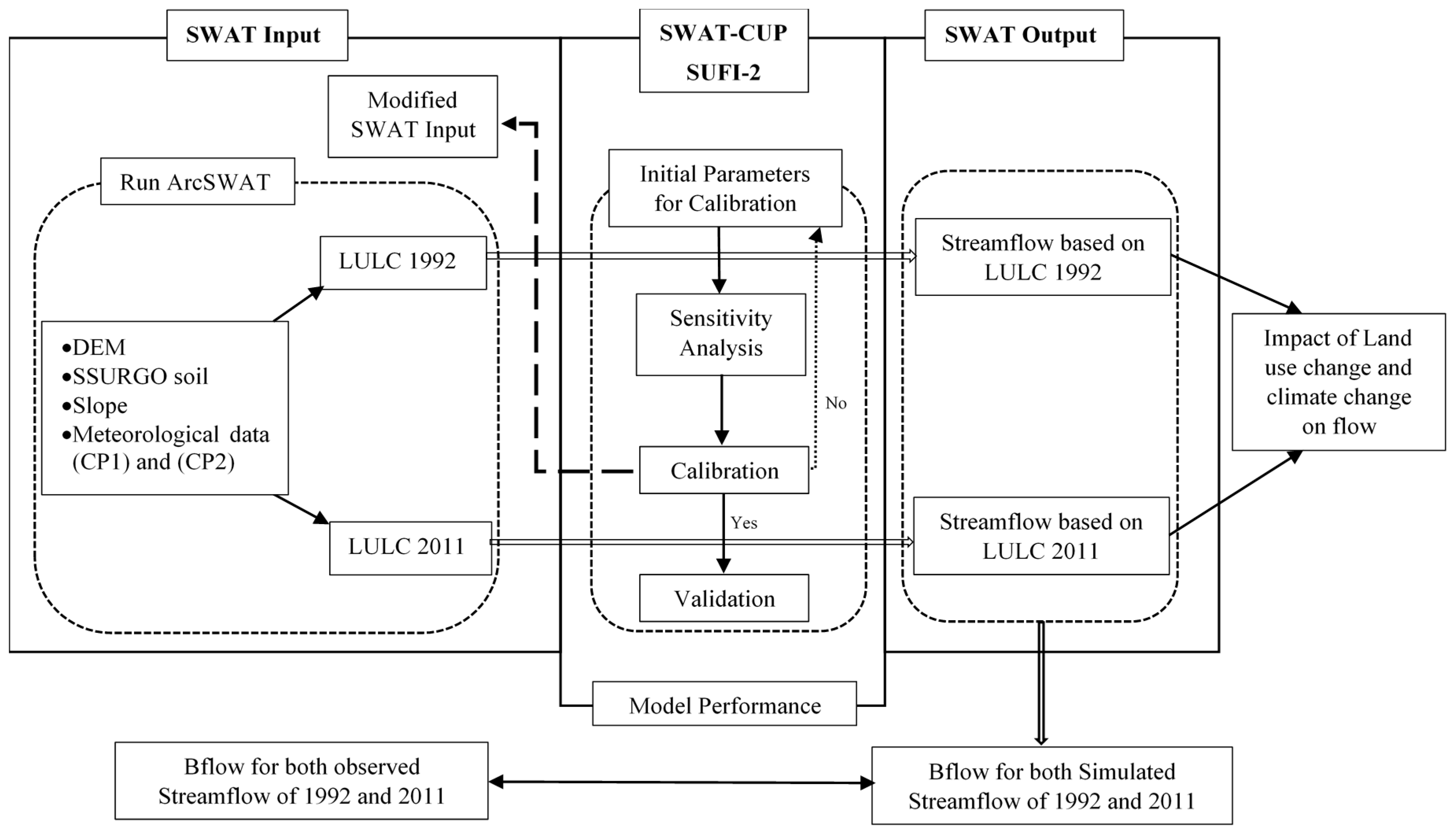
A flow chart of the model set up, sensitivity analysis, calibration and validation process of the streamflow and baseflow for the LEC watershed is described and summarized in Figure 2.
3. Results and Discussion
3.1. Land Use Changes from 1992 to 2011
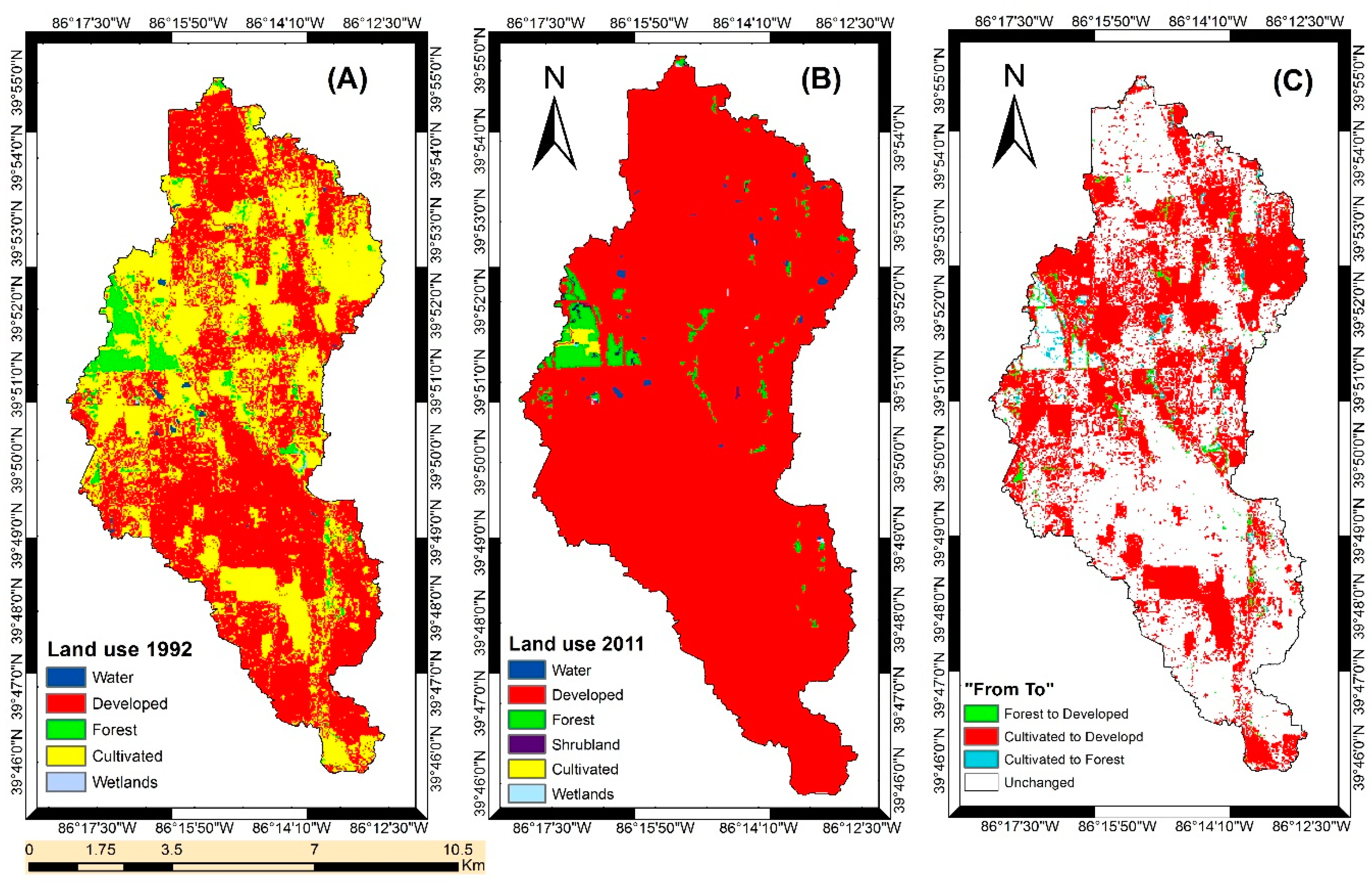
The 1992 and 2011 land use maps for the LEC watershed are shown in Figure 3A,B, and the change in land use types is shown in Figure 3C. The most commonly distributed land use types in LEC are developed and cultivated areas. Results highlighted from the land use change detection showed two clearly recognizable trends; (a) the decline of cultivated areas; and (b) rapid increase in developed areas. Developed areas showed an increase of 30.75 km2 or 75.8%. On the other hand, cultivated surface experienced a reduction of 30.16 km2 or 99.1% from 1992 to 2011.
Table 1 explains the variation in the LEC from 1992 to 2011 by analyzing the transition matrix of land use. 40.4 km2 of urban area remained unchanged, whereas the most notable transition is the conversion of 29.3 km2 of cultivated areas and 1.50 km2 of forests to urban uses from 1992 to 2011. The transition between other land uses was very small and have been omitted from analysis and the map. For instance, the change from water to developed and planted to water are only 0.14 and 0.16 km2, respectively. This might be attributed to the different classification algorithms used in NLCD data of 1992 and 2011.
3.2. Changes in Temperatures and Precipitation
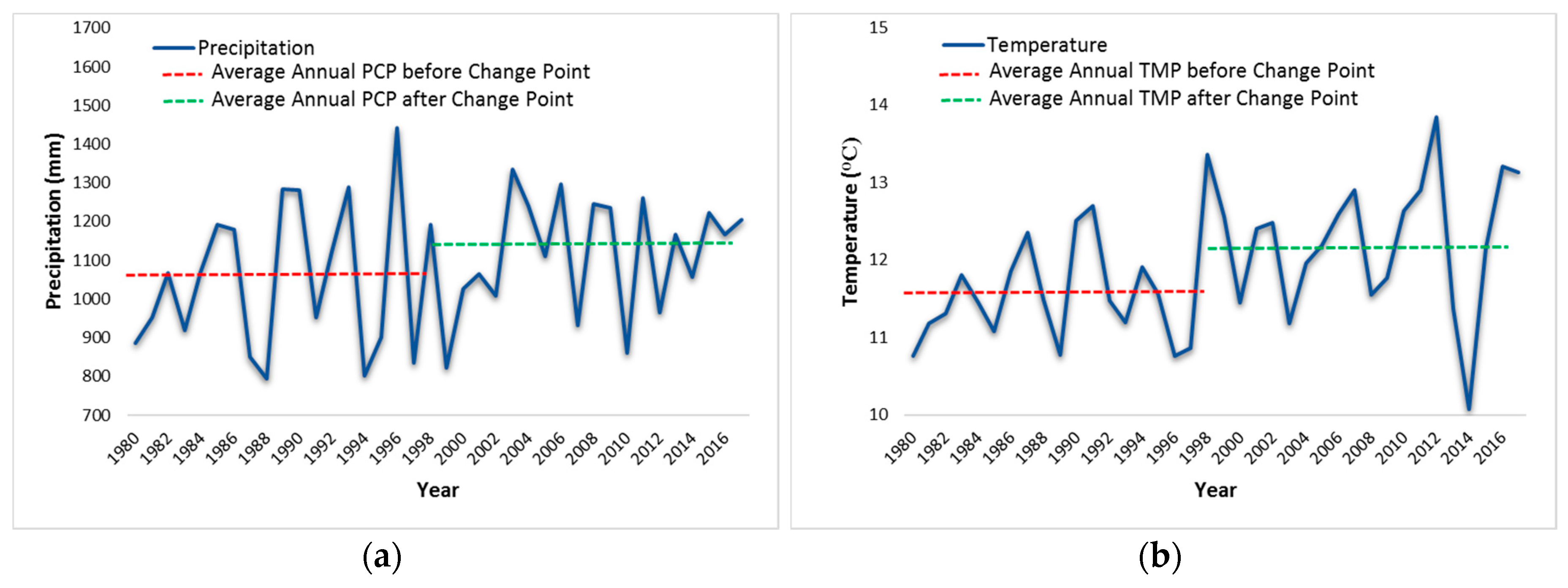
Both annual precipitation and temperature experienced a significant increase during the past 38 years. In order to quantify the magnitude of the increase in the meteorological data, the non-parametric M-K test was applied. The analysis showed that the meteorological time series data were not stationary, and there was one change point in the time series that occurred in 1998. This change is likely associated with regional environmental change such as urbanization and climate variability.
The trend Z-test statistics and the slope of precipitation and temperature were all positive and are displayed in Table 2. The results show that the monotonic trends of annual precipitation and temperature were different. For the overall period from 1980 to 2017, the annual precipitation increased at significance levels greater than 0.1, while air temperature passed the 0.001 significance level. These findings mean that the long-term monotonic trend of annual temperature exhibited a significant increase during the study period, whereas the long-term monotonic trend of annual precipitation is statistically insignificant and weak over time. Of note, statistical significance, or lacking of significance with respect to climate can be misleading. Although increase in annual temperature and precipitation were obtained, changes in seasonal precipitation and temperature might impact the increase in precipitation and temperature during the study period. For instance, Sekaluvu et al. [66] reported an overall insignificant decrease in precipitation by 0.4 mm/year during the period 2005–2015; however, winter and fall precipitation decreased by approximately 7.8 mm/year and 5.4 mm/year, respectively, and that reduction was significant. While spring precipitation increased significantly by 20 mm/year, and summer precipitation decreased insignificantly by about 4.0 mm/year.
Figure 4 shows the average values of annual precipitation and temperature before (red dashed line) and after (green dashed line) the change point. Compared to CP1, the results show that the average annual precipitation increased by 6.8% (73.7 mm, from 1080 mm to 1154 mm), while air temperature increased by 0.6 °C (from 11.6 °C to 12.2 °C) in the LEC.
In some cases, annual temperature and precipitation might not provide a true picture for the change in trends given the change in seasonality. Therefore, taking α = 0.05 as the significance level, the Mann–Kendal test was conducted at a monthly scale for the monthly precipitation and temperature data series. The outcomes showed a significant, positive, monotonic trend in the monthly precipitation in January and June in the LEC, while the monthly temperature exhibited a significant increase in April and September (Table 3).
3.3. Changes in Hydrological Variables
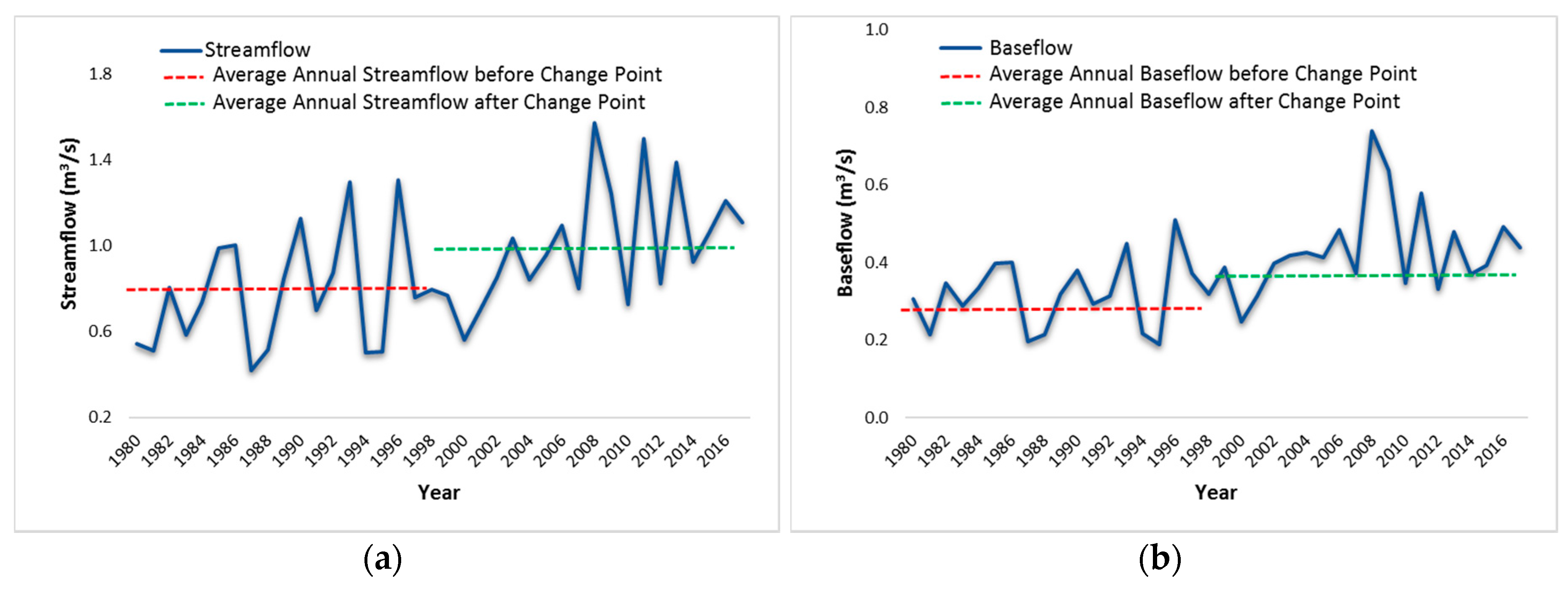
The monotonic trends of streamflow and baseflow in the LEC watershed were quantified using the Mann–Kendall test. The Z-statistics and the slope of annual streamflow and baseflow were positive (Table 4). Both long-term annual streamflow and baseflow in LEC were positively trending and significant at a level of 0.001; this implies that both showed significant increasing trends over the 1980–2017 period (Figure 5).
The increases in streamflow have a relationship with the increased rainfall. The increasing trend in annual baseflow might seem contradictory at first, as urbanization and imperviousness is increasing, the surface runoff is expected to increase instead of baseflow and infiltration. However, with a conductive hydrologic and geologic setting, evapotranspiration reductions, meeting water supply needs in urban areas and import of water into watersheds, sewage leakage, water distribution lines, retention and detention basins can all contribute to the baseflow to be increased in urban watersheds [40]. Detention basins have vital roles in increasing baseflow in urban watersheds, as water retained at the surface due to an increasing portion of surface runoff, and then slowly released into the stream as a form of baseflow. Therefore, increasing measures to maintain storm water over time may be a main reason for the increase of groundwater and baseflow in urban watersheds [67].
3.4. The SUFI-2 Calibration and Uncertainty Analysis Algorithm
The Sequential Uncertainty Fitting program algorithm (SUFI-2) approach within the SWAT-CUP interface was applied for optimization, calibration, validation and uncertainty analysis of parameters in the model [68]. In this algorithm, several sources of uncertainties, such as conceptual model, measured data (e.g., observed flow, sediments), driving variables (e.g., precipitation) and parameters, were quantified by the 95 Percent Prediction Uncertainty (95PPU), that calculate the cumulative distribution of an output variable at the 2.5% and 97.5% levels achieved through Latin Hypercube Sampling (LHS).
Based on previous studies, 20 hydrologic parameters were considered (Table 5). These parameters were described according to their existence among the main flow rate variable calibration parameters [51]. SUFI-2 begins with wide ranges of meaningful parameters that capture most of the observed data within the 95PPU and then iteratively decreases the uncertainty of the parameters [69]. Newer and narrower parameter ranges of uncertainties are computed after each iteration, in which larger uncertainty reductions are more related to the sensitive parameters [70]. Finally, the best fitted parameters obtained from SUFI-2 were incorporated into SWAT for streamflow and baseflow simulations at a daily time step but summarized monthly [49].
Performance assessment of the default model showed discrepancies between observed and simulated values; therefore, both automatic and manual calibration were done. Due to the large number of parameters within the SWAT model, a sensitivity analysis was first conducted, in order to decrease the number of parameters to be optimized. The calibration process included only sensitive parameters, and parameters were optimized based on monthly values [50].
The SUFI-2 global sensitivity analysis, in concurrence with the calibration procedure, was used to test 20 recommended parameters. Global sensitivity is important in identifying the relative significance of each parameter and the objective function sensitivity using the t-test. As a statistical measurement, the t-stat and p-value were used. A t-stat provides a sensitivity measure, in which greater absolute values are more sensitive, while the p-value determines the importance of the sensitivity [70].
Following Moriasi et al. [71], graphical comparison and statistical indices can assess the performance of the calibrated parameters. The coefficient of determination (R2), Nash–Sutcliffe model efficiency (ENS), PBIAS and modified Kling–Gupta Efficiency (KGE) were used to evaluate the model performance for the simulated streamflow and baseflow. The formulas for R2 and ENS, PBIAS and KGE can be acquired as previously outlined by Gupta et al. [72] and Nie et al. [73], respectively, and can be calculated as follows:
where
and
is the observed data, is the simulated output, and are the mean of the observed and simulated flow, respectively, r is the correlation between the measured and simulated values, β is the ratio between the simulated mean () and the observed mean () flow, and γ is the variation coefficient ration between the simulated () and the observed () flow, in which and represent the standard deviations of both simulated and measured data, respectively. Calibration and validation results were utilized to evaluate model success. Table 6 reports a model performance rating of “Very good, good, satisfactory and unsatisfactory” for each parameter.
3.5. Parameter Sensitivity Analysis
In this research, Little Eagle Creek data at the Speedway gauging station were used to calibrate the model. The threshold for defining HRUs were set as zero percent for soil, land and slope. The overlay of soil and land use maps, in addition to the slope percentage resulted in 516 HRUs, distributed over seven sub-basins. The sensitive parameters were optimized using the extension of auto-calibration in SWAT2012 to calibrate the hydrological model, and were recognized on the basis of global sensitivity analysis. Most of the parameters were modified on a trial and error basis within reasonable limits after consideration of the physical properties of the watershed. The global sensitivity analysis showed that parameters representing surface runoff, soil properties, and groundwater return flow are sensitive. Hence, it is important to accurately estimate these parameters for streamflow simulation. The 10 most sensitive input parameters are shown in Table 7, while the remaining parameters had less significant effect on streamflow simulation. Different ranks have been commonly detected in the same parameter for different watersheds and with a different number of simulations, which indicates the stochastic nature of SWAT-CUP [49].
For the LEC watershed, SUFI-2 outlined the most sensitive parameters to input changes, and these were ALPHA_BF, CN2, CH_K2, CH_N2, SOL_AWC, RCHRG_DP, EPCO, SMTMP, SFTMP, and CANMX. They each have a p-value close to zero. The ALPHA_BF and CN2, ranked first and second in sensitivity, respectively, and higher than the others which appeared to have made the most contribution in improving the ENS. In general, CN2, ALPHA_BF, SOL_AWC, and RCHRG_DP were important parameters for both baseflow and streamflow simulation, as the water traveling from the root zone in SWAT to deep aquifers was not redistributed into the main channel, soil, or shallow aquifers, but considered lost from the system boundary [76]. The high ALPHA_BF constant in the LEC watershed indicated a rapid response to groundwater recharge.
3.6. Selection of SWAT Model Structure
After incorporating all the data inputs, and in accordance with the detection of temporal trends in temperature and precipitation results, the period of 1980–2017 was divided into two time-spans, 1980–1998 and 1999–2017. The model was run for 1980–1998 with the first 4 years (1980–1983) used as a warm up period for the model. On the basis of the 1992 land use map, the period of 1980–1998 was recognized as the baseline condition for the SWAT model. The 1980–1993 period was assigned for model calibration, while the years from 1994–1998 were used for model validation. Careful consideration was be taken so that both calibration and validation periods have similar water balance [37]. The monthly statistical streamflow and baseflow outputs for the baseline model were used to evaluate the model performance.
3.7. Calibration and Validation of SWAT Model
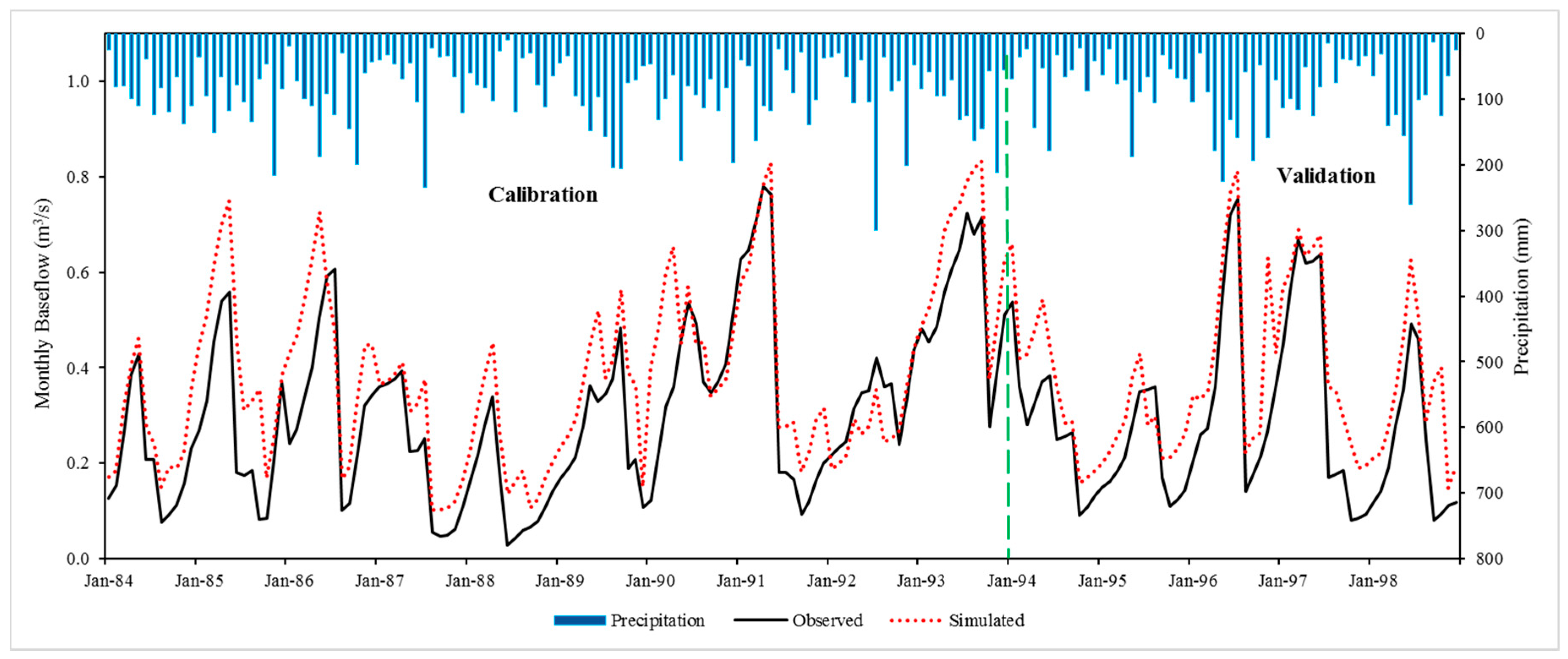
The proportion of baseflow (ratio of baseflow over total streamflow) of the measured and simulated streamflow are 36.5% and 39.1%, respectively. The good match indicated that partitioning between baseflow and surface runoff can be represented by the calibrated model in the LEC watershed [73].
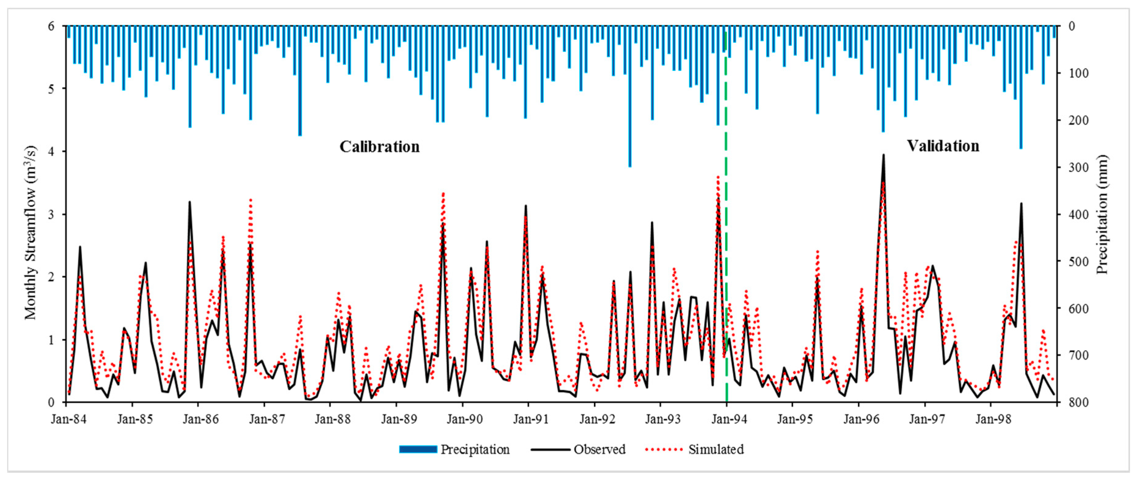
Figure 6 and Figure 7 show the simulated and measured monthly streamflow and baseflow for LEC during the calibration period (1984–1993) and validation period (1994–1998), with the first four years assigned as a warm up period (1980–1983). Model assessment statistics for monthly simulated streamflow and baseflow are summarized in Table 8. The ENS and R2 were 0.84 and 0.87, respectively, within the calibration period of streamflow, and 0.74 and 0.83 over the course of the validation period. These statistical outputs indicated that the simulated streamflow in calibration and validation were in ‘Very Good’ agreement, according Moriasi et al. [71] criteria.
As shown in Figure 6, observed and simulated streamflow outputs had a similar trend; in addition, the simulated streamflow showed a reasonable match with the observed records. Therefore, most of the measured and simulated streamflow values were bracketed by the 95 PPU, therefore, indicating comparatively little uncertainty for the streamflow simulation [70]. However, the relatively low agreements at the end of winter of some years could be explained by the model deficiency in capturing certain hydrological processes such as soil freezing-thawing and snowmelt during this period. In addition, some differences were observed in the peaks of observed and simulated values. These might have been due to the precipitation pattern or due to the limitations of the curve number (CN) method, as the CN method used in SWAT does not consider the duration and intensity of precipitation [73]. Results showed that the CN method overestimated streamflow for some large rainfall events. Overall, the observed and simulated average annual streamflow during the baseline model period was 0.83 m3/s and 0.98 m3/s, respectively.
The agreement between the measured and simulated streamflow during the calibration and validation period, to some extent, involves a good groundwater discharge simulation. The computed baseflow agreed well with the observed results for the LEC (Figure 7). During the calibration period, the R2, PBIAS, ENS and KGE were 0.80, −24.97, 0.60 and 0.67, respectively, while they were 0.84, −31.40, 0.58 and 0.58 for model validation (Table 8). The performance of the SUFI-2 model for baseflow simulation was considered ‘Good’ for calibration and ‘Satisfactory’ for validation, according to Moriasi et al. [71] and Moriasi et al. [77]. However, the peak baseflow was not well matched, as the SWAT simulation tended to overestimate baseflow, likely because of the spatial distribution of precipitation data is unevenly represented. In addition, peak baseflow may be attributed to the change in land use that influences hydrological phenomena and is related to direct runoff as well. An alternative possibility for the differences might be the presence of practices like surface detention and retention basins, in addition to the effect of soil freezing/thawing on infiltration and recharge during initial snowmelt. Overall, the average annual baseflow during the period from 1984 to 1998 for both measured and simulated data was 0.30 m3/s and 0.38 m3/s, respectively. These results ensure that the model can be further applied to assess hydrologic response analysis to various land use and climate change scenarios. Of note, despite the good agreements between the observed and simulated results, some uncertainty is associated with any hydrologic model [26]. Uncertainties in hydrologic models can arise from many different sources, including the structure of the conceptual model itself, initial conditions, parameters, observed input data, and interaction processes. However, the study area covers only 74.5 km2, and the amount of intense urbanization in which the watershed undergone may create some uncertainties, such as the surface water model not fully accounting for the complicated infrastructure in urbanized watersheds. Moreover, only 20 parameters were used to calibrate the model. Duan et al. [26] suggest that these may not be sufficient to represent. In addition, hydraulic conductivity can affect groundwater response time; however, most of the parameters in the SWAT model are surface-related such as hydraulic conductivity, saturated soil zones and channels. These parameters have been used in the calibrated baseline model to obtain an estimate of baseflow, but this assumes that the recharge of groundwater comes only from shallow aquifers to allow quicker contribution to baseflow. Additionally, SWAT divides underground storage into shallow and deep aquifers. The shallow aquifer receives recharge from unsaturated soil percolation. However, surface water models like SWAT hypothesize that water entering deep aquifers is considered lost from the system and therefore is not considered in future water budgets.
3.8. Changes in Total Water Yield and Baseflow within Various Simulation Scenario
Table 9 demonstrates the simulated SWAT annual average water yield and baseflow under different land use climate changes scenarios, as discussed in Section 2.3.4, in the LEC watershed. Results indicated that the difference in average annual water yield between S2 and S1, that simulated the impacts of land use change, showed an increase of 30.5 mm (6.7%). Meanwhile, the average annual water yield increased by 88.1 mm (17.9%) in S3 as compared to S1, which indicated the impacts of climate variability. Water yield increased by 91.9 mm (20.3%) due to the combined effects of land use change and climate variation; i.e., the contrast between S1 and S4. These findings indicated that the average annual water yield increased in the LEC during CP1 and CP2 due to the effects of both land use dynamics and climate variation, with the influences of climate change greater than that of the land use alteration. Meanwhile, the contribution of the combined impacts was higher than that of land use change and climate change separately. Therefore, the results emphasized that when climate variation played a dominant role, the impact of land use dynamics on water yield was not obvious. However, urban expansion also had a considerable impact on annual water yield by increasing impervious area, therefore, increasing surface runoff and decreasing water infiltration [78].
On the other hand, simulation suggested the reduction of the average annual baseflow due to the effect of land use change and the combined impacts of land use and climate change by an amount of 42.2 mm (28.8%) and 33.7 mm (23.0%), respectively, while the average annual baseflow increased by an amount of 22.3 mm (15.2%) due to the separate effects of climate change. Therefore, both land use change and the combined effects of land use and climate change had a greater negative impact on average annual baseflow, which illustrates the higher effect of land use change on baseflow on the LEC watershed. Climate variation has reduced the negative impact of land use change by 5.8%, as it increased from −28.8% to −23.0% from S2 to S4. The reduction of average annual baseflow in S2 and S4 may be because of several activities, for instance, over-exploitation, industrial uses, water withdrawal and groundwater pumping that are primarily used in the LEC watershed for production, manufacturing and daily human consumption. In addition, the decreasing trend seen in average annual baseflow could be due to the increase in surface runoff and lower soil infiltration, due to urbanization and increasing imperviousness that resulted in less water reaching unsaturated soils.
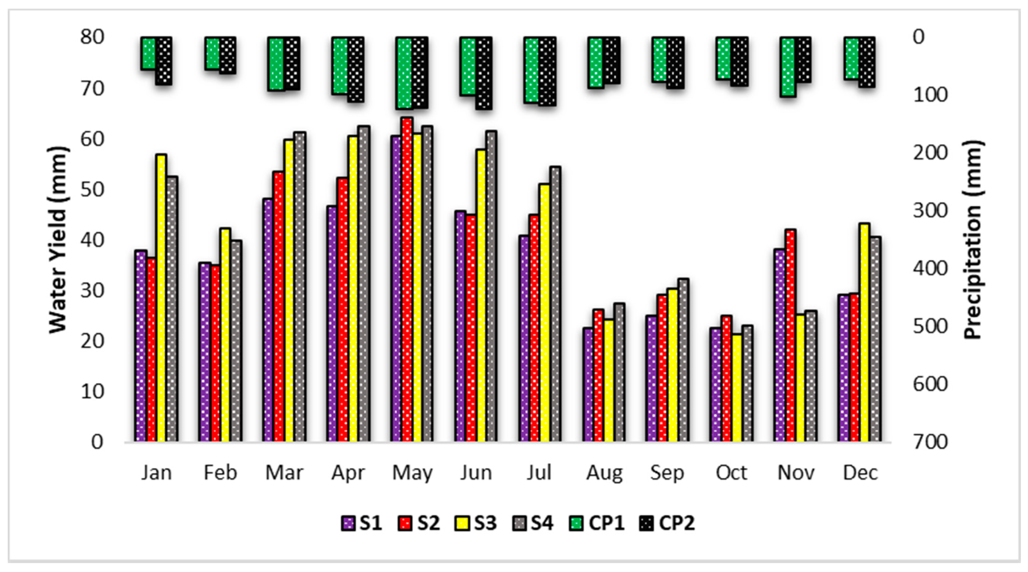
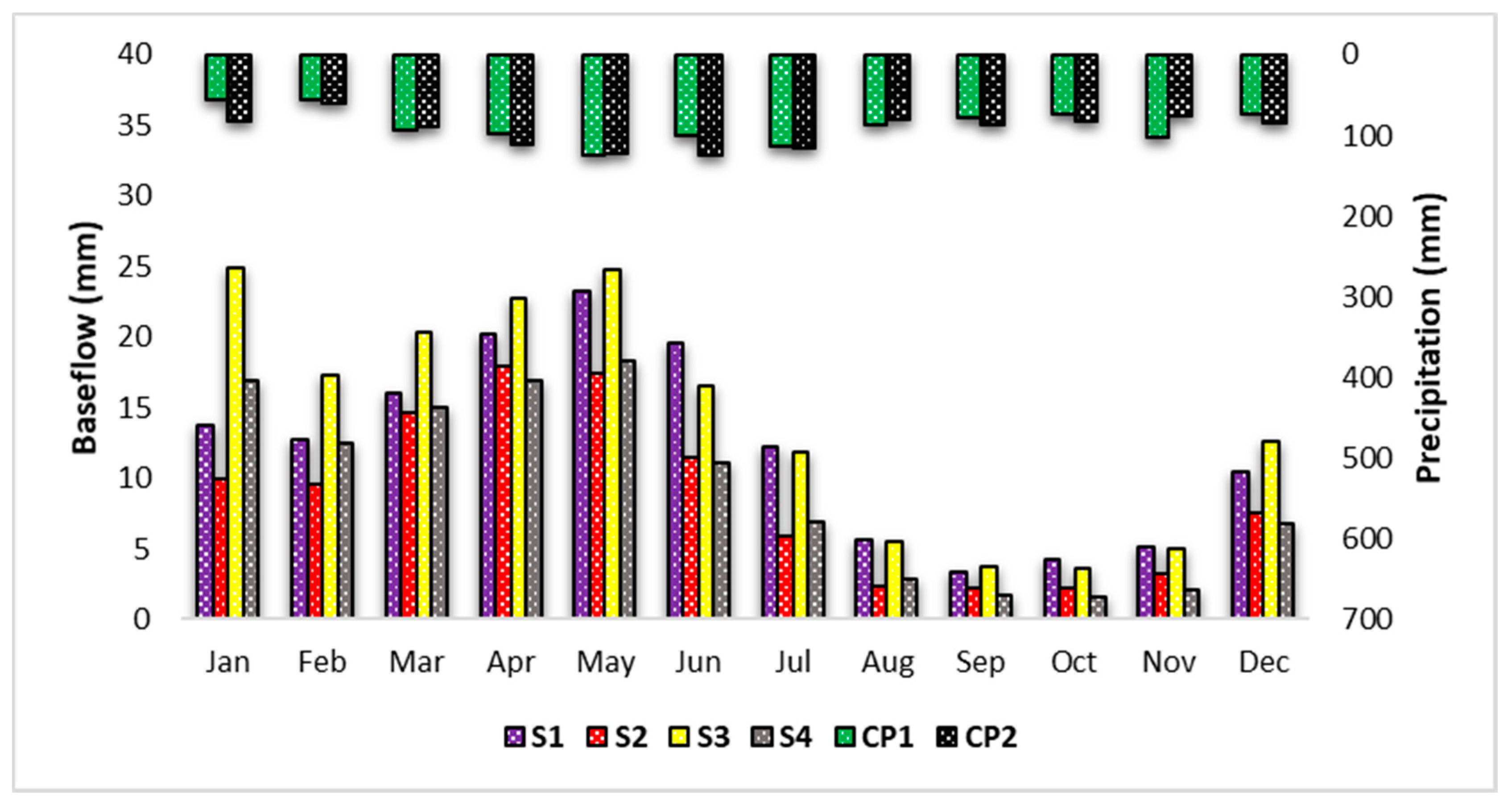
Figure 8 and Figure 9 show the results of the LEC watershed average monthly water yield and baseflow in different simulated scenarios. Most of the water yield was concentrated from March to July in all scenarios, i.e., within the rainy season. However, water yields accounted for 50% in both S1 and S2, while increasing to 55% in S3 and S4 during the rainy season. After evaluating the change in monthly precipitation between CP1 and CP2 (Figure 8), it might be concluded that the rainfall increase between CP1 and CP2 and the change in the pattern of average annual rainfall resulted in increased flood peaks between the two periods. The combined effects of climate variability and land use change drive an increase in monthly water yield in all months except November, which experienced a higher rainfall pattern in the first time period (CP1) as compared to CP2. Meanwhile, the average monthly baseflow response showed a similar behavior to the water yield response; however, the effect of climate change on baseflow was higher than the impact on water yield in the rainy season (Figure 9). Overall, both climate change and land use change had a greater impact on baseflow than water yield. Furthermore, average monthly baseflow showed an increase under the effect of solely climate change impacts of S3 in all months for the LEC watershed except for July and October, which showed a very minor reduction in baseflow (Figure 9). The highest average monthly increase occurred in the coldest months of the year with respect to S3 with the lowest amount of rainfall. This might be attributed to the process of freeze-thaw that can change the runoff process, soil infiltration and subsurface water storage. Therefore, baseflow from shallow aquifers considered the main contributor to total streamflow with the reduction of average monthly precipitation.
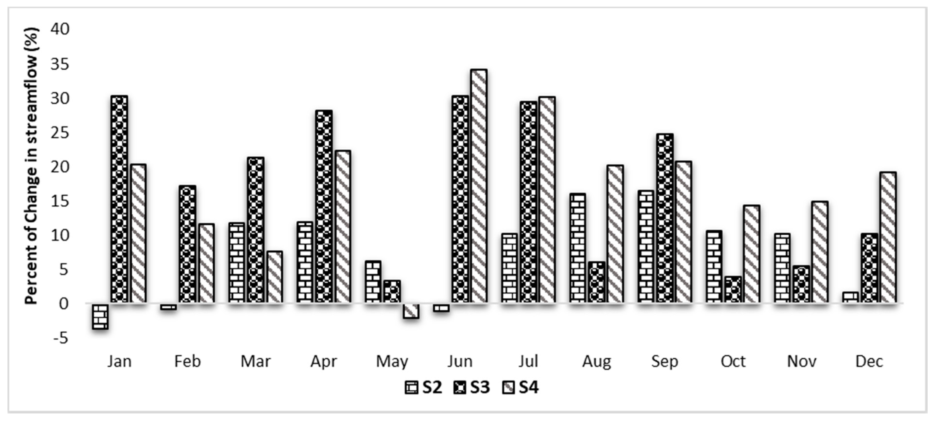
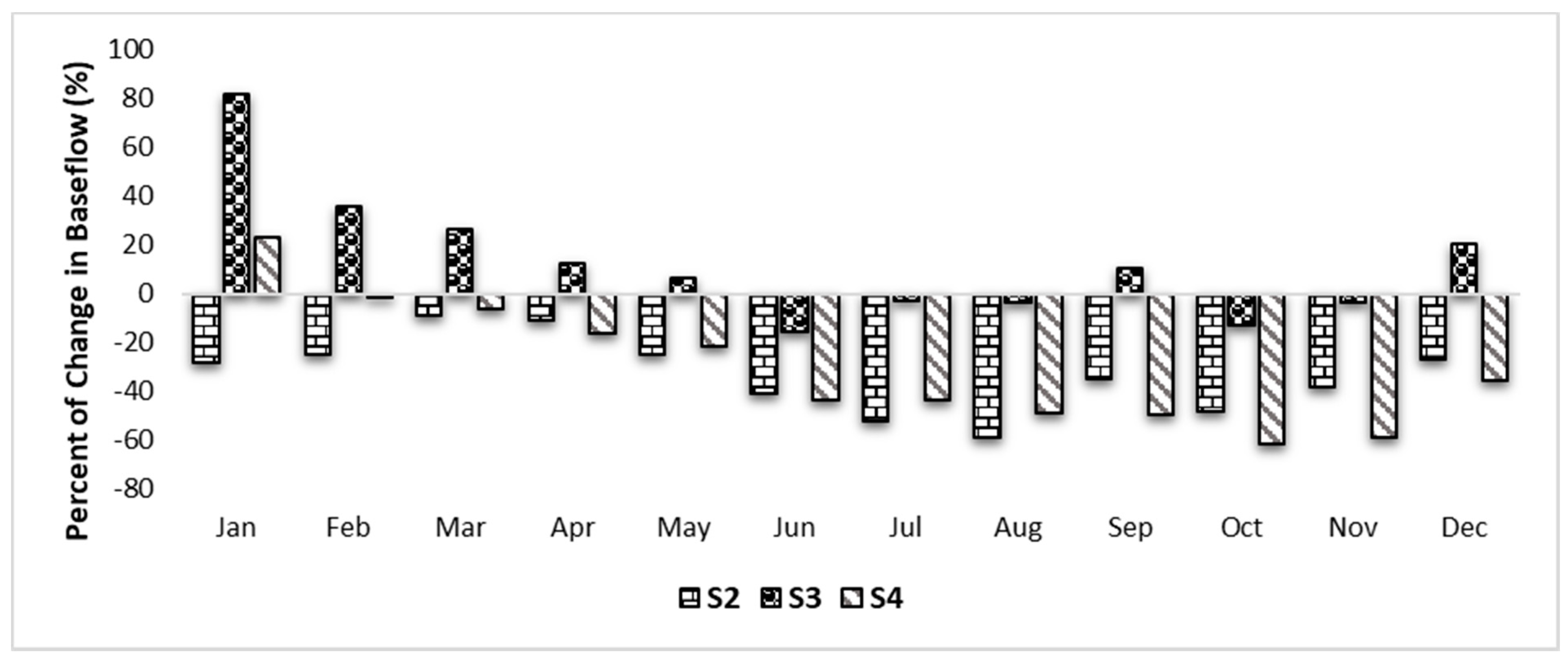
Figure 10 shows the average monthly streamflow changes relative to the baseline scenario (S1). Under the S2 scenario, the streamflow showed a reduction in January, February and June by 0.8% to 3.7%, while it increased in other months by 1.6 to 16.5%. Under the S3 scenario, however, streamflow showed an increase in all months, especially in summer, by an amount of 3.4% to 30.3%. Furthermore, the S4 scenario showed a similar trend in streamflow increase in all months by an amount ranging from 7.6% to 34.2%, with the only reduction recorded in May by 2.1%. On the other hand, Figure 11 shows the average monthly absolute changes in baseflow relative to the S1 (baseline) scenario. At the monthly timescale, baseflow showed a reduction in all months with respect to the S2 scenario (land use change) from 8.9% in March to the greatest reduction in August by 58.7%. A significant increase of baseflow occurred in all months ranging from 6.6% to 81.9% under the climate variation scenario (S3), while baseflow decreased with respect to the baseline scenario in the wet season by 2.9% to 15.5%. Finally, the S4 scenario showed reductions in baseflow for nearly the whole year ranging from 1.3% to 61.8%, while the only increase was found in January by 23.1%. Generally, the impact of the combined effects of land use and climate variation are reduced when the land use and climate variation cause changes in opposite directions. This can be clearly seen in all months of the year with respect to baseflow variation (Figure 9).
These changes in streamflow and baseflow were intimately bound up with the variation of precipitation between the two time periods. As can be seen in Figure 8 and Figure 9, the variation in precipitation generally reflects the variation in water yield in most months. However, the exception in other months may be attributed to the impacts of temperature fluctuation. For example, baseflow declined in October under the S3 scenario even with the increase in rainfall. That was possibly in connection with temperature rise in CP2 compared to CP1 [5], which could lead to an increase in evapotranspiration. In addition, compensatory contributors to baseflow, for example lawn irrigation, may contribute to this fundamental change in baseflow; therefore, a reduction in lawn irrigation might lead to the decline in the amount of water discharged to the shallow aquifer that contributed to baseflow.
4. Summary and Conclusions
Recognizing the impacts of land use alteration and climate variability on hydrologic systems is the basis for pragmatic watershed sustainability and ecological restoration efforts. In this study, the impacts of climate variability and land use change from 1980 to 2017 on water streamflow and baseflow in the Little Eagle Creek watershed have been evaluated using the non-parametric Mann–Kendall statistical test, land use maps and hydrologic modeling. The novelty lies in that not only were the effects of climate variation on hydrological response investigated, but the combined impact of land use dynamics and climate variation was also evaluated in an urbanized watershed in the US Midwest.
The long-term streamflow and baseflow response to land use change and climate variability were evaluated using the calibrated SWAT model. The model contained four scenarios in two periods, and applied two land use datasets (1992 and 2011) for the two climate periods (CP1 and CP2). By simulating the historical, continuous variation in streamflow, the SWAT model was calibrated and validated over the period 1980 to 1998 throughout the SUFI-2 approach within the SWAT-CUP interface. The SUFI-2 algorithm played an important role in minimizing the differences between measured and simulated streamflow in the LEC watershed. Discrepancies observed between the outputs of the model simulation and the observed data may in part occur due to the lack of meteorological input data from more than a single station. The SWAT model produced ‘very good’ and ‘good’ results for calibrating and validating observed streamflow and baseflow data. Hence, the calibrated parameters in this study can be used to carry out further future environmental and hydrological studies in similar watersheds. The hydrological balance assessment has shown that baseflow is a key component of the total discharge as it accounted for 36.5% of total flow within the LEC watershed. In general, SWAT proved versatile in modeling the effects of environmental changes in urban watersheds.
The model was used to explore likely impacts of urbanization and climate variation in an urban watershed. Much of the original cultivated and forest areas had already been converted to developed areas or urbanization. During the period of 1992–2011, about 39% of the LEC watershed area changed from cultivated to urban areas, while the climate became warmer and wetter. Overall, climate variability had the dominant impact on streamflow, while urban expansion influenced baseflow more significantly than climate change. Urbanization can be considered a major environmental stressor controlling hydrological components, including surface runoff, baseflow, and water yield in a catchment. Understanding the variation in streamflow and baseflow due to the separate and coupled effects of climate variation and land use dynamics is essential for sustainable management of water resources. The results gleaned from this study can be useful in providing information for management and planning of water resources, in addition to assessing the prospective impacts of adaptation measures to cope with climate variation, particularly in areas that are sensitive to climate variability and experiencing high urbanization.
The results obtained in this study must be interpreted carefully, with the caveat that the meteorological station records reflect data that are the result of the combined impacts of land use alteration and climate variability. Since these affects cannot be separated in this data, the predicted impact of climate variability alone on streamflow and baseflow may not be simulated accurately. Studies that focus on quantifying the effect of each land use category change on streamflow and baseflow are likely to yield useful additional insights on how climate variability and land use impact hydrological response separately. Furthermore, additional studies using catchments that exhibit different urbanization and climate regions could provide beneficial comparative results to determine the impacts of these variables on hydrological components.
Supplementary Materials
The following are available online at https://www.mdpi.com/2073-4441/11/8/1603/s1, Hydro-Meteorological Data.
Author Contributions
Writing-original draft, M.A.; Methodology, M.A.; Formal analysis, M.A. and B.A.E.; Editing-review M.W.G. and B.A.E.; Conceptualization M.W.G.; Supervision B.A.E.
Funding
This research was funded by Egyptian Government General Scholarship Programme (Ministry of Higher Education), administrated by the Egyptian Cultural and Education Bureau, Washington, DC, USA (Call 2013/2014).
Acknowledgments
The authors would like to thank Celena Alford and Erin Sorlien for their critical reviews of the manuscript, and the Egyptian Government for financial support through the General Scholarship Program.
Conflicts of Interest
The authors declare no conflicts of interest.
References
- Abdi, R.; Yasi, M. Evaluation of environmental flow requirements using eco-hydrologic-hydraulic methods in perennial rivers. Water Sci. Technol. 2015, 72, 354–363. [Google Scholar] [CrossRef] [PubMed]
- Wang, X.; Engel, B.; Yuan, X.; Yuan, P. Variation analysis of streamflows from 1956 to 2016 along the Yellow River, China. Water 2018, 10, 1231. [Google Scholar] [CrossRef]
- Kibria, K.; Ahiablame, L.; Hay, C.; Djira, G. Streamflow Trends and Responses to Climate Variability and Land Cover Change in South Dakota. Hydrology 2016, 3, 2. [Google Scholar] [CrossRef]
- Duan, W.; Chen, Y.; Zou, S.; Nover, D. Managing the water-climate- food nexus for sustainable development in Turkmenistan. J. Clean. Prod. 2019, 220, 212–224. [Google Scholar] [CrossRef]
- Zhang, L.; Nan, Z.; Yu, W.; Ge, Y. Modeling Land-Use and Land-Cover Change and Hydrological Responses under Consistent Climate Change Scenarios in the Heihe River Basin, China. Water Resour. Manag. 2015, 29, 4701–4717. [Google Scholar] [CrossRef]
- Guo, J.; Zhang, Z.; Zhou, J.; Wang, S.; Strauss, P. Decoupling Streamflow Responses to Climate Variability and Land Use/Cover Changes in a Watershed in Northern China. J. Am. Water Resour. Assoc. 2014, 50, 1425–1438. [Google Scholar] [CrossRef]
- Zheng, H.; Zhang, L.; Zhu, R.; Liu, C.; Sato, Y.; Fukushima, Y. Responses of streamflow to climate and land surface change in the headwaters of the Yellow River Basin. Water Resour. Res. 2009, 45, 1–9. [Google Scholar] [CrossRef]
- Omer, A.; Wang, W.; Basheer, A.K.; Yong, B. Integrated assessment of the impacts of climate variability and anthropogenic activities on river runoff: A case study in the Hutuo River Basin, China. Hydrol. Res. 2017, 48, 416–430. [Google Scholar] [CrossRef]
- Park, J.Y.; Park, M.J.; Joh, H.K.; Shin, H.J.; Kwon, H.J.; Srinivasan, R.; Kim, S.J. Assessment of MIROC 3.2 HiRes Climate and CLUE-s Land Use Change Impacts on Watershed Hydrology Using SWAT. Trans. ASABE 2011, 54, 1713–1724. [Google Scholar] [CrossRef]
- Shi, P.; Ma, X.; Hou, Y.; Li, Q.; Zhang, Z.; Qu, S.; Chen, C.; Cai, T.; Fang, X. Effects of Land-Use and Climate Change on Hydrological Processes in the Upstream of Huai River, China. Water Resour. Manag. 2013, 27, 1263–1278. [Google Scholar] [CrossRef]
- Tong, S.T.Y.; Sun, Y.; Ranatunga, T.; He, J.; Yang, Y.J. Predicting plausible impacts of sets of climate and land use change scenarios on water resources. Appl. Geogr. 2012, 32, 477–489. [Google Scholar] [CrossRef]
- Tao, X.E.; Chen, H.; Xu, C.Y.; Hou, Y.K.; Jie, M. xuan Analysis and prediction of reference evapotranspiration with climate change in Xiangjiang River Basin, China. Water Sci. Eng. 2015, 8, 273–281. [Google Scholar] [CrossRef]
- Zhang, Y.; Engel, B.; Ahiablame, L.; Liu, J. Impacts of climate change on mean annual water balance for watersheds in Michigan, USA. Water 2015, 7, 3565–3578. [Google Scholar] [CrossRef]
- Kim, J.; Choi, J.; Choi, C.; Park, S. Impacts of changes in climate and land use/land cover under IPCC RCP scenarios on streamflow in the Hoeya River Basin, Korea. Sci. Total Environ. 2013, 452–453, 181–195. [Google Scholar] [CrossRef]
- Duan, W.; He, B.; Nover, D.; Fan, J.; Yang, G.; Chen, W.; Meng, H.; Liu, C. Floods and associated socioeconomic damages in China over the last century. Nat. Hazards 2016, 82, 401–413. [Google Scholar] [CrossRef]
- Zhang, D.; Liu, X.; Liu, C.; Bai, P. Responses of runoff to climatic variation and human activities in the Fenhe River, China. Stoch. Environ. Res. Risk Assess. 2013, 27, 1293–1301. [Google Scholar] [CrossRef]
- Xu, X.; Scanlon, B.R.; Schilling, K.; Sun, A. Relative importance of climate and land surface changes on hydrologic changes in the US Midwest since the 1930s: Implications for biofuel production. J. Hydrol. 2013, 497, 110–120. [Google Scholar] [CrossRef]
- Tu, J. Combined impact of climate and land use changes on streamflow and water quality in eastern Massachusetts, USA. J. Hydrol. 2009, 379, 268–283. [Google Scholar] [CrossRef]
- Fohrer, N.; Haverkamp, S.; Eckhardt, K.; Frede, H.-G. Hydrologic Response to Land Use Changes on the Catchment Scale. Pergamon Phys. Chem. Earth B 2001, 26, 577–582. [Google Scholar] [CrossRef]
- Novotny, E.V.; Stefan, H.G. Stream flow in Minnesota: Indicator of climate change. J. Hydrol. 2007, 334, 319–333. [Google Scholar] [CrossRef]
- Kumar, S.; Merwade, V.; Kam, J.; Thurner, K. Streamflow trends in Indiana: Effects of long term persistence, precipitation and subsurface drains. J. Hydrol. 2009, 374, 171–183. [Google Scholar] [CrossRef]
- Frans, C.; Istanbulluoglu, E.; Mishra, V.; Munoz-Arriola, F.; Lettenmaier, D.P. Are climatic or land cover changes the dominant cause of runoff trends in the Upper Mississippi River Basin? Geophys. Res. Lett. 2013, 40, 1104–1110. [Google Scholar] [CrossRef]
- Tan, M.L.; Ibrahim, A.L.; Yusop, Z.; Duan, Z.; Ling, L. Impacts of land-use and climate variability on hydrological components in the Johor River basin, Malaysia. Hydrol. Sci. J. 2015, 60, 1–17. [Google Scholar] [CrossRef]
- Wang, W.; Shao, Q.; Yang, T.; Peng, S.; Xing, W.; Sun, F.; Luo, Y. Quantitative assessment of the impact of climate variability and human activities on runoff changes: A case study in four catchments of the Haihe River basin, China. Hydrol. Process. 2013, 27, 1158–1174. [Google Scholar] [CrossRef]
- Zou, S.; Jilili, A.; Duan, W.; De Maeyer, P.; Van de Voorde, T. Human and natural impacts on thewater resources in the Syr Darya River Basin, Central Asia. Sustainability 2019, 11, 3084. [Google Scholar] [CrossRef]
- Duan, W.; He, B.; Takara, K.; Luo, P.; Nover, D.; Hu, M. Impacts of climate change on the hydro-climatology of the upper Ishikari river basin, Japan. Environ. Earth Sci. 2017, 76, 1–16. [Google Scholar] [CrossRef]
- Khoi, D.N.; Thom, V.T. Impacts of climate variability and land-use change on hydrology in the period 1981-2009 in the central highlands of vietnam. Glob. Nest J. 2015, 17, 870–881. [Google Scholar]
- Li, Z.; Liu, W.Z.; Zhang, X.C.; Zheng, F.L. Impacts of land use change and climate variability on hydrology in an agricultural catchment on the Loess Plateau of China. J. Hydrol. 2009, 377, 35–42. [Google Scholar] [CrossRef]
- Jothityangkoon, C.; Sivapalan, M.; Farmer, D.L. Process controls of water balance variability in a large semi-arid catchment: Downward approach to hydrological model development. J. Hydrol. 2001, 254, 174–198. [Google Scholar] [CrossRef]
- Legesse, D.; Vallet-Coulomb, C.; Gasse, F. Hydrological response of a catchment to climate and land use changes in Tropical Africa: Case study south central Ethiopia. J. Hydrol. 2003, 275, 67–85. [Google Scholar] [CrossRef]
- Lu, Z.; Zou, S.; Xiao, H.; Zheng, C.; Yin, Z.; Wang, W. Comprehensive hydrologic calibration of SWAT and water balance analysis in mountainous watersheds in northwest China. Phys. Chem. Earth 2015, 79–82, 76–85. [Google Scholar] [CrossRef]
- Beven, K. A manifesto for the equifinality thesis. J. Hydrol. 2006, 320, 18–36. [Google Scholar] [CrossRef] [Green Version]
- Rusli, N.; Majid, M.R.; Yusop, Z.; Tan, M.L.; Hashim, S.; Bohari, S.N. Integrating manual calibration and auto-calibration of SWAT model in Muar Watershed, Johor. In Proceedings of the 2016 7th IEEE Control and System Graduate Research Colloquium (ICSGRC), Shah Alam, Malaysia, 8 August 2016; pp. 197–202. [Google Scholar]
- Duan, W.; Hanasaki, N.; Shiogama, H.; Chen, Y.; Zou, S.; Nover, D.; Zhou, B.; Wang, Y. Evaluation and future projection of Chinese precipitation extremes using large ensemble high-resolution climate simulations. J. Clim. 2019, 32, 2169–2183. [Google Scholar] [CrossRef]
- Setegn, S.G.; Srinivasan, R.; Dargahi, B. Hydrological Modelling in the Lake Tana Basin, Ethiopia Using SWAT Model. Open Hydrol. J. 2008, 2, 49–62. [Google Scholar] [CrossRef] [Green Version]
- Arnold, J.G.; Srinivasan, R.; Muttiah, R.S.; Williams, J.R. Large area hydrologic modeling and assesment Part I: Model development. JAWRA J. Am. Water Resour. Assoc. 1998, 34, 73–89. [Google Scholar] [CrossRef]
- Arnold, J.G.; Moriasi, D.N.; Gassman, P.W.; Abbaspour, K.C.; White, M.J.; Srinivasan, R.; Santhi, C.; Harmel, R.D.; Van Griensven, A.; Van Liew, M.W.; et al. SWAT: Model Use, Calibration, and Validation. Trans. ASABE 2012, 55, 1491–1508. [Google Scholar] [CrossRef]
- Huang, X.D.; Shi, Z.H.; Fang, N.F.; Li, X. Influences of land use change on baseflow in mountainous watersheds. Forests 2016, 7, 16. [Google Scholar] [CrossRef]
- Abbaspour, K.C.; Rouholahnejad, E.; Vaghefi, S.; Srinivasan, R.; Yang, H.; Kløve, B. A continental-scale hydrology and water quality model for Europe: Calibration and uncertainty of a high-resolution large-scale SWAT model. J. Hydrol. 2015, 524, 733–752. [Google Scholar] [CrossRef] [Green Version]
- Ahiablame, L.; Chaubey, I.; Engel, B.; Cherkauer, K.; Merwade, V. Estimation of annual baseflow at ungauged sites in Indiana USA. J. Hydrol. 2013, 476, 13–27. [Google Scholar] [CrossRef]
- McIntyre, N.; Ballard, C.; Bruen, M.; Bulygina, N.; Buytaert, W.; Cluckie, I.; Dunn, S.; Ehret, U.; Ewen, J.; Gelfan, A.; et al. Modelling the hydrological impacts of rural land use change. Hydrol. Res. 2014, 45, 737–754. [Google Scholar] [CrossRef]
- Bhaduri, B.; Harbor, J.; Engel, B.; Grove, M. Assessing watershed-scale, long-term hydrologic impacts of land-use change using a GIS-NPS model. Environ. Manag. 2000, 26, 643–658. [Google Scholar] [CrossRef]
- Grove, M.; Harbor, J.; Engel, B.; Muthukrishnan, S. Impacts of urbanization on surface hydrology, Little Eagle Creek, Indiana, and analysis of LTHIA model sensitivity to data resolution. Phys. Geogr. 2001, 22, 135–153. [Google Scholar] [CrossRef]
- Doyle, M.W.; Harbor, J.M.; Rich, C.F.; Spacie, A.B. Examining the effects of urbanization on streams using indicators of geomorphic stability. Phys. Geogr. 2000, 21, 37–41. [Google Scholar] [CrossRef]
- Choi, J.; Engel, B.A.; Muthukrishnan, S.; Harbor, J. GIS Based Long Term Hydrologic Impact Evaluation for Watershed Urbanization. J. Am. Water Resour. Assoc. 2003, 2051, 623–635. [Google Scholar] [CrossRef]
- Tang, Z.; Engel, B.A.; Lim, K.J.; Pijanowski, B.C.; Harbor, J. Minimizing the impact of urbanization on long term runoff. J. Am. Water Resour. Assoc. 2005, 41, 1347–1359. [Google Scholar] [CrossRef]
- Lim, K.J.; Engel, B.A.; Muthukrishnan, S.; Harbor, J. Effects of initial abstraction and urbanization on estimated runoff using CN technology. J. Am. Water Resour. Assoc. 2006, 42, 629–643. [Google Scholar] [CrossRef]
- Lim, K.J.; Engel, B.A.; Tang, Z.; Muthukrishnan, S.; Choi, J.; Kim, K. Effects of calibration on L-THIA GIS runoff and pollutant estimation. J. Environ. Manag. 2006, 78, 35–43. [Google Scholar] [CrossRef]
- Mehan, S.; Neupane, R.P.; Kumar, S. Coupling of SUFI 2 and SWAT for Improving the Simulation of Streamflow in an Agricultural Watershed of South Dakota. Hydrol. Curr. Res. 2017, 8. [Google Scholar] [CrossRef]
- Welde, K.; Gebremariam, B. Effect of land use land cover dynamics on hydrological response of watershed: Case study of Tekeze Dam watershed, northern Ethiopia. Int. Soil Water Conserv. Res. 2017, 5, 1–16. [Google Scholar] [CrossRef]
- Almeida, R.A.; Pereira, S.B.; Pinto, D.B.F. Calibration and Validation of the SWAT Hydrological Model for the Mucuri River Basin. Eng. Agrícola 2018, 4430, 55–63. [Google Scholar] [CrossRef]
- Neitsch, S.L.; Arnold, J.G.; Kiniry, J.R.; Williams, J.R. Soil and Water Assessment Tool User’s Manual. Version 2005. 2005, pp. 1–494. Available online: https://swat.tamu.edu/media/1292/SWAT2005theory.pdf (accessed on 21 June 2018).
- Wallace, C.W.; Flanagan, D.C.; Engel, B.A. Evaluating the effects ofwatershed size on SWAT calibration. Water 2018, 10, 898. [Google Scholar] [CrossRef]
- Neitsch, S.L.; Arnold, J.G.; Kiniry, J.R.; Srinivasan, R.; Williams, J.R. Soil and Water Assessment Tool User’s Manual Version 2000. TWRI Rep. TR-192. 2002, pp. 1–412. Available online: https://swat.tamu.edu/media/1294/swatuserman.pdf (accessed on 21 June 2018).
- Aboelnour, M.; Engel, B.A. Application of Remote Sensing Techniques and Geographic Information Systems to Analyze Land Surface Temperature in Response to Land Use/Land Cover Change in Greater Cairo Region, Egypt. J. Geogr. Inf. Syst. 2018, 10, 57–88. [Google Scholar] [CrossRef] [Green Version]
- Gitau, M.; Bailey, N. Multi-Layer Assessment of Land Use and Related Changes for Decision Support in a Coastal Zone Watershed. Land 2012, 1, 5–31. [Google Scholar] [CrossRef] [Green Version]
- Gitau, M.W.; Chaubey, I.; Gbur, E.; Pennington, J.H.; Gorham, B. Impacts of land-use change and best management practice implementation in a Conservation Effects Assessment Project watershed: Northwest Arkansas. J. Soil Water Conserv. 2010, 65, 353–368. [Google Scholar] [CrossRef] [Green Version]
- Hamed, K.H.; Rao, R.A. A modified Mann-Kendall trend test for autocorrelated data. J. Hydrol. 1998, 204, 182–196. [Google Scholar] [CrossRef]
- Kendall, M.G. Rank Correlation Methods, 4th ed.; Charles Griffin: London, UK, 1975. [Google Scholar]
- Tesemma, Z.K.; Mohamed, Y.A.; Steenhuis, T.S. Trends in rainfall and runoff in the Blue Nile Basin: 1964–2003. Hydrol. Process. 2010, 24, 3747–3758. [Google Scholar] [CrossRef]
- Sen, P.K. Estimates of the Regression Coefficient Based on Kendall’s Tau. J. Am. Stat. Assoc. 1968, 63, 1379–1389. [Google Scholar] [CrossRef]
- Hirsch, R.M.; Slack, J.R.; Smith, R.A. Techniques of trend analysis for monthly water quality data. Water Resour. Res. 1982, 18, 107–121. [Google Scholar] [CrossRef] [Green Version]
- Jung, Y.; Shin, Y.; Won, N.I.; Lim, K.J. Web-based BFlow system for the assessment of streamflow characteristics at national level. Water 2016, 8, 384. [Google Scholar] [CrossRef]
- Lee, J.; Kim, J.; Jang, W.S.; Lim, K.J.; Engel, B.A. Assessment of baseflow estimates considering recession characteristics in SWAT. Water 2018, 10, 371. [Google Scholar] [CrossRef]
- Eckhardt, K. A comparison of baseflow indices, which were calculated with seven different baseflow separation methods. J. Hydrol. 2008, 352, 168–173. [Google Scholar] [CrossRef]
- Sekaluvu, L.; Zhang, L.; Gitau, M. Evaluation of constraints to water quality improvements in the Western Lake Erie Basin. J. Environ. Manag. 2018, 205, 85–98. [Google Scholar] [CrossRef]
- Meyer, S.C. Analysis of base flow trends in urban streams, Northeastern Illinois, USA. Hydrogeol. J. 2005, 13, 871–885. [Google Scholar] [CrossRef]
- Abbaspour, K.C. SWAT-CUP: SWAT Calibration and Uncertainty Programs. 2015, Volume 130. Available online: https://swat.tamu.edu/media/114860/usermanual_swatcup.pdf (accessed on 10 October 2018).
- Neitsch, S.; Arnold, J.; Kiniry, J.; Williams, J. Soil & Water Assessment Tool Theoretical Documentation; Version 2009; Texas Water Resources Institute: College Station, TX, USA, 2011; pp. 1–647. [Google Scholar]
- Zuo, D.; Xu, Z.; Yao, W.; Jin, S.; Xiao, P.; Ran, D. Assessing the effects of changes in land use and climate on runoff and sediment yields from a watershed in the Loess Plateau of China. Sci. Total Environ. 2016, 544, 238–250. [Google Scholar] [CrossRef]
- Moriasi, D.N.; Arnold, J.G.; Van Liew, M.W.; Bingner, R.L.; Harmel, R.D.; Veith, T.L. Model Evaluation Guidelines for Systematic Quantification of Accuracy in Watershed Simulations. Trans. ASABE 2007, 50, 885–900. [Google Scholar] [CrossRef]
- Gupta, H.V.; Kling, H.; Yilmaz, K.K.; Martinez, G.F. Decomposition of the mean squared error and NSE performance criteria: Implications for improving hydrological modelling. J. Hydrol. 2009, 377, 80–91. [Google Scholar] [CrossRef] [Green Version]
- Nie, W.; Yuan, Y.; Kepner, W.; Nash, M.S.; Jackson, M.; Erickson, C. Assessing impacts of Landuse and Landcover changes on hydrology for the upper San Pedro watershed. J. Hydrol. 2011, 407, 105–114. [Google Scholar] [CrossRef]
- Moriasi, D.N.; Gowda, P.H.; Arnold, J.G.; Mulla, D.J.; Ale, S.; Steiner, J.L.; Tomer, M.D. Evaluation of the Hooghoudt and Kirkham Tile Drain Equations in the Soil and Water Assessment Tool to Simulate Tile Flow and Nitrate-Nitrogen. J. Environ. Qual. 2013, 42, 1699. [Google Scholar] [CrossRef]
- Thirel, G.; Andréassian, V.; Perrin, C.; Audouy, J.N.; Berthet, L.; Edwards, P.; Folton, N.; Furusho, C.; Kuentz, A.; Lerat, J.; et al. Hydrologie sous changement: Un protocole d’évaluation pour examiner comment les modèles hydrologiques s’accommodent des bassins changeants. Hydrol. Sci. J. 2015, 60, 1184–1199. [Google Scholar] [CrossRef]
- Jang, W.S.; Engel, B.; Ryu, J. Efficient flow calibration method for accurate estimation of baseflow using a watershed scale hydrological model (SWAT). Ecol. Eng. 2018, 125, 50–67. [Google Scholar] [CrossRef]
- Moriasi, D.N.; Gitau, M.W.; Pai, N.; Daggupati, P. Hydrologic and Water Quality Models: Performance Measures and Evaluation Criteria. Trans. ASABE 2015, 58, 1763–1785. [Google Scholar] [Green Version]
- Zhao, A.; Zhu, X.; Liu, X.; Pan, Y.; Zuo, D. Impacts of land use change and climate variability on green and blue water resources in the Weihe River Basin of northwest China. Catena 2015, 137, 318–327. [Google Scholar] [CrossRef]
Figure 1.
Index map showing location of the Little Eagle Creek (LEC) watershed in Indiana.

Figure 2.
Flow chart depicting procedure for SWAT model setup, calibration and validation of both streamflow and baseflow in the LEC watershed.
Figure 2.
Flow chart depicting procedure for SWAT model setup, calibration and validation of both streamflow and baseflow in the LEC watershed.

Figure 3.
Land use types in LEC watershed in (A) 1992; (B) 2011 and (C) the transition between 1992 and 2011.
Figure 3.
Land use types in LEC watershed in (A) 1992; (B) 2011 and (C) the transition between 1992 and 2011.

Figure 4.
Annual precipitation (a) and temperature (b) in the LEC watershed.

Figure 5.
Average daily streamflow (a) and baseflow (b) over time in the LEC watershed.

Figure 6.
Observed and simulated streamflow of LEC watershed for calibration and validation period.

Figure 7.
Observed and simulated baseflow of LEC watershed for calibration and validation period.

Figure 8.
Average monthly water yield for the LEC watershed under different scenarios.

Figure 9.
Average monthly baseflow for the LEC watershed under different scenarios.

Figure 10.
Relative change in average monthly streamflow in the LEC watershed.

Figure 11.
Relative change in average monthly baseflow in the LEC watershed.


Table 1.
Land use change transition matrix in LEC from 1992 to 2011 (km2).
| 1992 | 2011 | ||||||
|---|---|---|---|---|---|---|---|
| Water | Developed | Forest | Shrubland | Cultivated | Wetlands | Total | |
| Water | 0.10 | 0.14 | 0 | 0 | 0 | 0 | 0.25 |
| Developed | 0.05 | 40.38 | 0.15 | 0.01 | 0 | 0.02 | 40.62 |
| Forest | 0.01 | 1.50 | 1.59 | 0.07 | 0.03 | 0.01 | 3.21 |
| Cultivated | 0.16 | 29.34 | 0.62 | 0 | 0.24 | 0.02 | 30.38 |
| Wetlands | 0 | 0.04 | 0 | 0 | 0 | 0 | 0.05 |
| Total | 0.33 | 71.41 | 2.36 | 0.08 | 0.27 | 0.05 | |
Table 2.
Temporal trends in annual precipitation and temperature in the LEC watershed.
| Precipitation | Temperature | |
|---|---|---|
| Z-Stat | 1.521 | 2.930 |
| Slope | 4.219 | 0.032 |
| α | >0.1 | 0.001 |
Table 3.
Trend analysis and significance test for monthly precipitation and temperature in the LEC Watershed.
Table 3.
Trend analysis and significance test for monthly precipitation and temperature in the LEC Watershed.
| Jan | Feb | Mar | Apr | May | Jun | Jul | Aug | Sep | Oct | Nov | Dec | |
|---|---|---|---|---|---|---|---|---|---|---|---|---|
| Precipitation | ||||||||||||
| Z-Stat | 2.238 | −0.352 | 0.402 | 1.308 | −0.214 | 2.226 | −0.063 | −0.038 | −0.013 | 0.780 | −0.478 | 0.339 |
| Slope | 1.167 | −0.037 | 0.206 | 1.216 | −0.116 | 2.055 | 0.243 | −0.321 | 0.194 | 0.290 | −0.834 | 0.153 |
| Sig | S | NS | NS | NS | NS | S | NS | NS | NS | NS | NS | NS |
| p-value | 0.006 | 0.181 | 0.172 | 0.048 | 0.208 | 0.006 | 0.237 | 0.242 | 0.247 | 0.109 | 0.158 | 0.184 |
| Temperature | ||||||||||||
| Z-Stat | 0.83 | 0.201 | 1.031 | 2.552 | 1.144 | 1.396 | −0.717 | 1.195 | 1.974 | 1.107 | 0.779 | 0.05 |
| Slope | 0.33 | 0.004 | 0.05 | 0.066 | 0.028 | 0.029 | −0.005 | 0.027 | 0.048 | 0.035 | 0.02 | 0.044 |
| Sig | NS | NS | NS | S | NS | NS | NS | NS | S | NS | NS | NS |
| p-value | 0.102 | 0.210 | 0.076 | 0.002 | 0.063 | 0.041 | 0.118 | 0.058 | 0.012 | 0.067 | 0.109 | 0.240 |
S: Significant. NS: Not significant. Significant level (α) = 0.05.
Table 4.
Temporal trends in annual streamflow and baseflow in the LEC watershed.
| Streamflow | Baseflow | |
|---|---|---|
| Z-Stat | 3.319 | 3.395 |
| Slope | 5.078 | 2.062 |
| α | 0.001 | 0.001 |
Table 5.
SWAT input parameters used for the LEC calibration of streamflow and baseflow.
| Parameter | Ext. | Description | Adjustment | IV | LB | UB | FV |
|---|---|---|---|---|---|---|---|
| Parameters controlling water balance | |||||||
| ESCO | hru | Soil evaporation compensation factor | R | 0.95 | 0.01 | 1 | 0.08 |
| EPCO | hru | Plant uptake compensation factor | R | 1 | 0.01 | 1 | 0.48 |
| CANMX | hru | Max canopy storage | R | 0 | 0 | 25 | 23.5 |
| SFTMP | bsn | Snowfall temp | R | 1 | −5 | 5 | −3.4 |
| SMTMP | bsn | Snowmelt base temp | R | 0.5 | −5 | 5 | 3.8 |
| TIMP | bsn | Snow back temp lag factor | R | 1 | 0.01 | 1 | 0.59 |
| SMFMX | bsn | Melt factor for snow on 21 June | R | 4.5 | 0.01 | 10 | 1.38 |
| SMFMN | bsn | Melt factor for snow on 21 December | R | 4.5 | 0.01 | 10 | 4.09 |
| Parameters controlling surface water response | |||||||
| CN2 | mgt | Initial SCS Curve number | V | -- | −0.25 | 0.25 | 0.22 |
| SURLAG | bsn | Surface runoff lag coefficient | R | 4 | 0.1 | 10 | 3.28 |
| Parameters controlling subsurface water response | |||||||
| ALPHA_BF | gw | Baseflow alpha factor | R | 0.048 | 0.01 | 1 | 0.75 |
| GWQMN | gw | Depth of water for return flow | R | 1000 | 0.01 | 5000 | 1273 |
| GW_DELAY | gw | Groundwater delay time | R | 31 | 0.1 | 50 | 19.4 |
| REVAPMN | gw | Depth of water for evaporation | R | 750 | 0.01 | 250 | 124 |
| GW_REVAP | gw | Groundwater evaporation coefficient | R | 0.02 | 0.02 | 0.2 | 0.15 |
| RCHRG_DP | gw | Deep aquifer percolation fraction | R | 0.05 | 0.01 | 1 | 0.59 |
| Parameters controlling soil’s physical properties | |||||||
| SOL_AWC | sol | Available water capacity of the soil water | V | -- | −0.25 | 0.25 | 0.10 |
| SOL_K | sol | Saturated hydraulic conductivity | V | -- | −0.15 | 0.15 | 0.03 |
| Parameters controlling channel’s physical properties | |||||||
| CH_K2 | rte | Effective hydraulic conductivity | R | 0 | 5 | 300 | 32.6 |
| CH_N2 | rte | Main channel manning | R | 0.014 | 0.01 | 0.15 | 0.08 |
Ext: Extension, R: Replace by value, V: Multiply by value, IV: Initial values, LB: Lower bound, UB: Upper bound, FV: Final value.
Table 6.
SWAT performance evaluation criteria according to Moriasi et al. [74], Thirel et al. [75], and Lee et al. [64].
| Measure | Output | Evaluation Criteria of the Model † | |||
|---|---|---|---|---|---|
| Very Good | Good | Satisfactory | Unsatisfactory | ||
| R2 | Flow | >0.85 | 0.75 < R2 < 0.85 | 0.60 < R2 < 0.75 | R2 ≤ 0.60 |
| ENS | Flow | >0.80 | 0.70 < ENS < 0.80 | 0.50 < ENS < 0.70 | ENS ≤ 0.50 |
| PBIAS | Flow | <±10 | ±10 ≤ PBIAS ≤ ±15 | ±15 ≤ PBIAS ≤ ±30 | PBIAS ≥ ±30 |
| KGE | Flow | >0.80 | 0.70 < KGE < 0.80 | 0.50 < KGE < 0.70 | KGE ≤ 0.50 |
Table 7.
List of top 10 ranking sensitive parameters for SWAT in the LEC watershed and their calibrated values.
Table 7.
List of top 10 ranking sensitive parameters for SWAT in the LEC watershed and their calibrated values.
| Rank | Parameter | Calibrated Value | t-Stat | p-Value |
|---|---|---|---|---|
| 1 | ALPHA_BF | 0.81 | 44.71 | 0 |
| 2 | CN2 | 0.02 | 18.47 | 0 |
| 3 | CH_K2 | 28.39 | −13.34 | 0 |
| 4 | CH_N2 | 0.08 | −4.72 | 0 |
| 5 | SOL_AWC | −0.17 | −4.13 | 0 |
| 6 | RCHRG_DP | 0.01 | −3.16 | 0 |
| 7 | EPCO | 0.16 | −2.99 | 0 |
| 8 | SMTMP | −1.51 | 2.48 | 0.01 |
| 9 | SFTMP | 4.90 | −2.24 | 0.03 |
| 10 | CANMX | 23.27 | 1.95 | 0.05 |
Table 8.
Values of statistical indicators in the calibration and validation periods for streamflow and baseflow in the LEC watershed.
Table 8.
Values of statistical indicators in the calibration and validation periods for streamflow and baseflow in the LEC watershed.
| Period | Streamflow (m3/s) | Baseflow (m3/s) | |||||||
|---|---|---|---|---|---|---|---|---|---|
| R2 | ENS | PBIAS | KGE | R2 | ENS | PBIAS | KGE | ||
| Calibration | (1984–1993) | 0.87 | 0.84 | −14.4 | 0.81 | 0.80 | 0.60 | −24.9 | 0.67 |
| Validation | (1994–1998) | 0.83 | 0.74 | −26.9 | 0.72 | 0.84 | 0.58 | −31.4 | 0.58 |
Table 9.
Average annual change in water yield and baseflow in the LEC watershed.
| Scenario | Land Use | Climate | Water Yield (mm) | Baseflow (mm) | Surface Runoff (mm) | ||||||
|---|---|---|---|---|---|---|---|---|---|---|---|
| Av. | Ch. Δ | (%) | Av. | Ch. Δ | (%) | Av. | Ch. Δ | (%) | |||
| S1 | NLCD 1992 | CP1 | 452.7 | - | - | 146.5 | - | - | 294.1 | - | - |
| S2 | NLCD 2011 | CP1 | 483.2 | 30.5 | 6.7 | 104.3 | −42.2 | −28.8 | 374.7 | 80.6 | 27.4 |
| S3 | NLCD 1992 | CP2 | 533.8 | 81.1 | 17.9 | 168.8 | 22.3 | 15.2 | 360.9 | 66.8 | 22.7 |
| S4 | NLDC 2011 | CP2 | 544.6 | 91.9 | 20.3 | 112.8 | −33.7 | −23.0 | 428.5 | 134.3 | 45.7 |
© 2019 by the authors. Licensee MDPI, Basel, Switzerland. This article is an open access article distributed under the terms and conditions of the Creative Commons Attribution (CC BY) license (http://creativecommons.org/licenses/by/4.0/).
Share and Cite
MDPI and ACS Style
Aboelnour, M.; Gitau, M.W.; Engel, B.A. Hydrologic Response in an Urban Watershed as Affected by Climate and Land-Use Change. Water 2019, 11, 1603. https://doi.org/10.3390/w11081603
AMA Style
Aboelnour M, Gitau MW, Engel BA. Hydrologic Response in an Urban Watershed as Affected by Climate and Land-Use Change. Water. 2019; 11(8):1603. https://doi.org/10.3390/w11081603
Chicago/Turabian StyleAboelnour, Mohamed, Margaret W. Gitau, and Bernard A. Engel. 2019. "Hydrologic Response in an Urban Watershed as Affected by Climate and Land-Use Change" Water 11, no. 8: 1603. https://doi.org/10.3390/w11081603
Note that from the first issue of 2016, this journal uses article numbers instead of page numbers. See further details here.