Impact of Pressure-Driven Demand on Background Leakage Estimation in Water Supply Networks


1
Department of Electrical Engineering, Tshwane University of Technology, Pretoria 0001, South Africa
2
École Supérieure d’Ingénieurs en Électrotechnique et Électronique, Cite Descartes, BP 99, Noisy-le-Grand, 93162 Paris, France
3
Council for Scientific and Industrial Research (CSIR), Pretoria 0184, South Africa
*
Author to whom correspondence should be addressed.
Water 2019, 11(8), 1600; https://doi.org/10.3390/w11081600
Submission received: 1 July 2019
/
Revised: 24 July 2019
/
Accepted: 29 July 2019
/
Published: 1 August 2019
(This article belongs to the Section Urban Water Management)
Abstract
:Increasing water demand due to urbanization creates a need to develop schemes for managing water supply networks (WSNs). In recent years, hydraulic modeling of WSNs has been used to assess the state of networks in terms of leakage analysis and pressure control. These models are based on demand-driven modeling (DDM) analysis and pressure-driven modeling (PDM) analysis. The former assumes that the nodal demand is fulfilled consistently regardless of the nodal pressure head. The latter appraises the demand as a function of the available pressure head at the nodes. In a previous paper by Adedeji et al. (2017), an algorithm was presented for background leakage detection and estimation in WSNs. The results demonstrated that the algorithm allows the detection of critical pipes and the indication of the nodes where such critical pipes are located for possible pressure control. However, such an algorithm assumes a demand-driven condition of WSNs. In this paper, a pressure-driven modeling is integrated into the developed algorithm with emphasis on its impact on the background leakage estimate. The results obtained are compared to the demand-driven analysis using two WSNs as case studies. The results presented, which consider pipe and node levels, demonstrate that the reliance of the nodal demand on the available pressure head at the node influences the magnitude of the background leakage flow. It is conceived that this investigation might be crucial for the background leakage estimation while considering WSNs operating under pressure-deficient conditions. In this paper, the solution time for both simulation scenarios is also presented.
1. Introduction
Supplying good quality drinking water to meet the ever-increasing consumer demand has become a major task for water utilities. This impels the need to perform water network asset management to evaluate the state of underground or above-ground water pipelines for system planning, schedule maintenance, loss reduction, and demand prediction purposes. In water distribution networks, water loss is a typical challenge to the operational services of water utilities. The problem associated with these losses is gargantuan in scale, thus, the need for cost-effective techniques for leakage detection has become an increasingly important area of research in recent years [1].
During recent decades, water utilities have received distinctive proposals to confine leakage in water supply frameworks. These are based on devices such as leak noise correlators, acoustic noise loggers, ground-penetrating radars, step testing, combined acoustic loggers and correlators, electronic step testers, digital correlators, and advanced ground microphones [1,2]. As of late, the acquisition of geographic information and supervisory control systems in the water industries has allowed the utilization of hydraulic models for investigating the condition of the water networks in near real-time. These investigations have been used, for example, for network design and optimization, leakage analysis, as well as pressure control for leakage minimization [3,4,5,6,7,8,9,10,11,12,13,14,15,16].
Most software packages used for water network simulation such as EPANET assume that the water demand at the nodes is fulfilled consistently regardless of the network nodal pressure. This presumption disentangles the problem, even though it is only legitimate for WSNs under normal operating conditions [17,18] where the pressure can be relied upon to satisfactorily fulfill the nodal demand. Nonetheless, practically speaking, a WSN behaves in such a way that if the pressure at a node falls beneath a base level because of some network events, for example, network failures or valve shut down, the flow from this node will significantly reduce, and in extreme cases, the discharge will become zero, irrespective of the actual demand [17]. Consequently, for some pressure-deficient WSNs, where the demand cannot be met at certain consumer nodes, integrating a pressure-driven modeling (PDM) into the hydraulic models of water networks would offer a pragmatic simulation.
In WSNs, background leakage is that of outflow from small cracks, and because these are characterized by a diffuse flow, they are difficult to detect using measuring instruments, they thus pose a threat to water utilities. The estimation of such leakage flow could prove valuable for reducing water loss volume in various water supply networks [19,20,21]. The aim of this paper is to integrate a PDM analysis into the algorithm in [21] and investigate its impact on the background leakage estimation in water supply networks. The analysis may be useful for leakage estimations in water networks under low-pressure conditions or areas of low-pressure occurrence in the network. The rest of the paper is organized as follows. The next section presents the overview of pressure-driven demand functions. In Section 2, the integration of the PDM and the background leakage model into the water network hydraulic formulation using graph theory is presented. Section 3 presents the analysis of the case study networks used as numerical examples, while Section 4 concludes the paper.
Overview of Pressure-Dependent Demand Functions
Numerous research attempts have been conducted to oversee the pressure-dependent demand (PDD) relationships. Among the notable PDD functions are the Heaviside step function proposed by Bhave [22] as expressed in Equation (1), the PDD function of Wagner et al. [23] and Chandapillai [24] shown in Equation (2), and that of Wu et al. [25] presented in Equation (3).
In these equations, , , and denote the pressure-dependent demand function, the demand, and the pressure head (the difference between the piezometric head and the elevation) at node i, respectively; while is the minimum nodal pressure head under which water cannot be supplied from node i; denotes the service pressure head necessary to fully satisfy the required demand at node i; and represents the threshold pressure head above which the demand is not dependent on the nodal pressure. Some other PDD relationships may be found in the literature [2,26,27,28,29].
Despite the numerous definitions of the pressure-dependent demand relationships, the function represented by Equation (2) is most broadly used and is adopted in this study. In this relationship, the pressure-dependent nodal demand () falls between zero and the desired service demand () depending on the state of the WSNs. In some cases where field data is not available, under which no water can be supplied by the node may be set as the ground elevation at each node [18]. Furthermore, below which the nodal demand cannot be completely satisfied may be carefully chosen to vary between 14 m to 15 m or more [30,31].
2. Methods
Integrating a PDD Function and Pressure-Dependent Leakage Modeling in the WSN Hydraulic Model Formulation
Any network, whether electrical, structural, water, or other fluid, can be represented in terms of topological matrices derived from the structure of the network. Take into account a WSN with number of pipes, number of nodes with unknown heads, and number of fixed-head nodes (nodes with known heads), in terms of network topological matrices, the flows and heads in the network may be represented by a system of equations as
where E is a diagonal matrix of dimensions () relating the head losses to the flow in each pipe as . Both h and are the head at the junction and fixed-head nodes, respectively. q and d are the vector of the unknown flow in each pipe and the demand at the junction nodes. of size () and of size () are the incidence sub-matrices with connecting the pipes to the junction nodes and connecting pipes to the fixed-head nodes. These two matrices are derived from the network incidence matrix A expressed as shown in Equation (A1).
To integrate a PDM, the demand vector in Equation (4) comprises the PDD function from Equation (2) and the pressure-dependent leakage model. Following similar procedure by Giustolisi et al. (2008), the pressure-dependent leakage relationship is defined in the vector of the nodal leakage flow rate. Therefore, Equation (4) may be rewritten as
where denotes the () vector of the pressure-dependent nodal leakage flow rate computed from the pipe leakage model (the vector of the pipe background leakage flow rate). Using the topological incidence matrix, both and are derived as shown in Equations (A2)–(A5).
Thus, it is possible to write Equation (5) conveniently as
The function may be solved using Newton–Raphson (NR) method based on the Jacobian of . The Jacobian matrix J of the function in Equation (6) may be expressed as shown in Equation (A6).
Therefore, when the Newton–Raphson method is applied to Equation (6) at each iteration “k”, the estimate of the nodal head and the flow in each pipe is given as
In a similar manner to the demand-driven modeling (DDM) analysis [21,32], the estimate of the head in this analysis is expressed as
The PDM formulation is very similar to the conventional demand-driven modeling (DDM) formulation as it may be noticed in Equation (7) and Equation (9), the only distinction lies within the appearance of and within the description of the nodal demand as pressure-dependent. Therefore, a PDM may be simply integrated into the DDM without any advanced mathematical formulations. All computations were done using MATLAB R2013a software; Mathworks, Massachusetts, United States, on a hp EliteBook 8560p computer with a 6 GB RAM and 64-bit operating system; HP Inc., Palo Alto, California, United States. A tolerance of [33] was used as the stoping criterion. The effect of the two hydraulic model simulation scenarios, the DDM analysis, and the PDM analysis on the background leakage estimation were compared and analyzed.
3. Results and Analysis
Numerical Examples
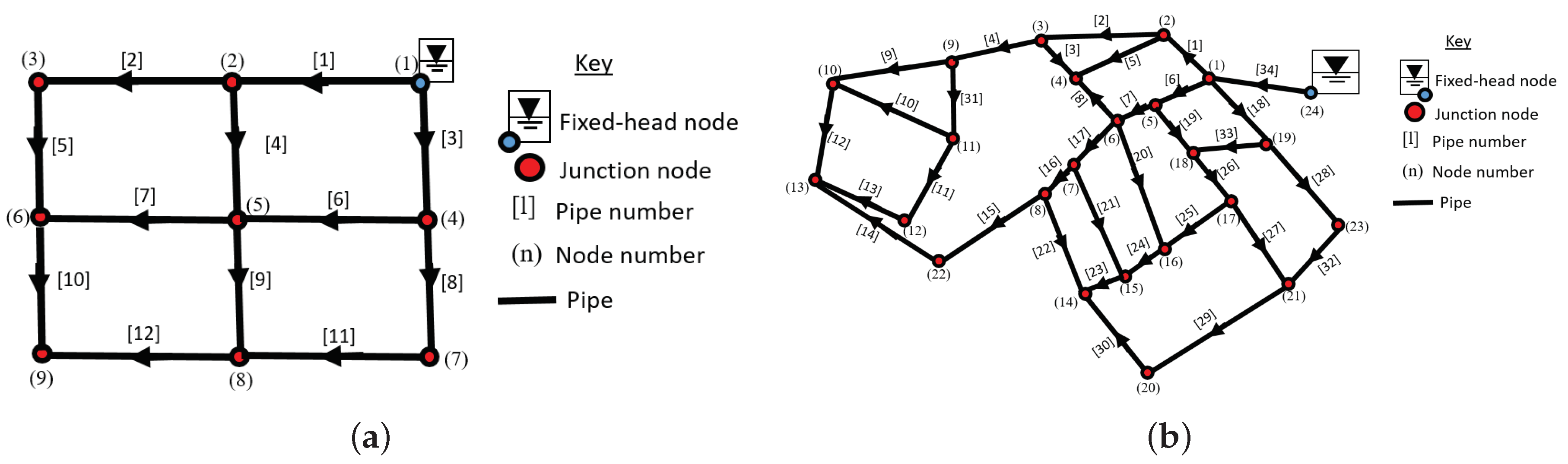
To realize the objective of this study, two WSNs (as illustrated in Figure 1) were used as case studies. [19] was assumed for both networks. In Figure 1a, schematics of the WSN used for the numerical example (Network 1) is presented. As observed in Figure 1a, the network consists of 12 pipes interconnected between nine nodes. An elevated reservoir which acts as a supply node is provided where the water is supplied by gravity at a head of 100 m. In addition, the pipes have a varying diameter from 100 mm to 250 mm while the demand at the nodes varies between 62.5 L/s to 208.1 L/s. The Hazen–Williams model is used for the head loss estimation. The Hazen–Williams coefficient for all the pipes is equal to 130. The data relating to the nodes and pipes of this network may be found in [29]. For this network, the PDM analysis was executed by setting the service pressure head to 10 m. The minimum pressure head below which no water can be supplied from the node was set to 0 m to perform the PDM scenario.
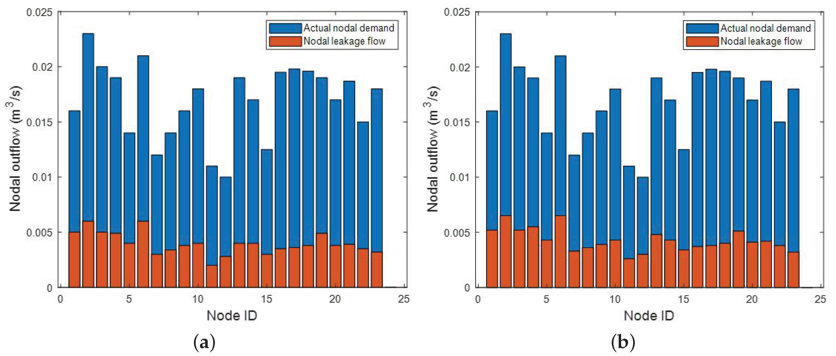
Figure 2 relays the profile of the nodal leakage flow with regard to the particular demand at the node for both simulation scenarios, i.e., DDM analysis (Figure 2a) and PDM analysis (Figure 2b) for network 1. In both scenarios, the magnitude of the background leakage flow in all the nodes is lower compared to the demand. The peak of the leakage flow is noticed in node 4, although with a slightly increased level for the PDM analysis (Figure 2b). A slight increment may be noticed in nodes 5, 6, 7, and 8 in Figure 2b as compared to the DDM case in Figure 2a. This is due to the relatively high pressure head status observed in the PDM when compared to the DDM case for this network. In addition, for both simulation scenarios, no leakage flow occurs in node 9. This is because node 9 is characterized by a negative pressure head. Furthermore, it is observed that for both scenarios, the profile of the leakage flow and the required demand follow a similar trend from node 2 to node 9.
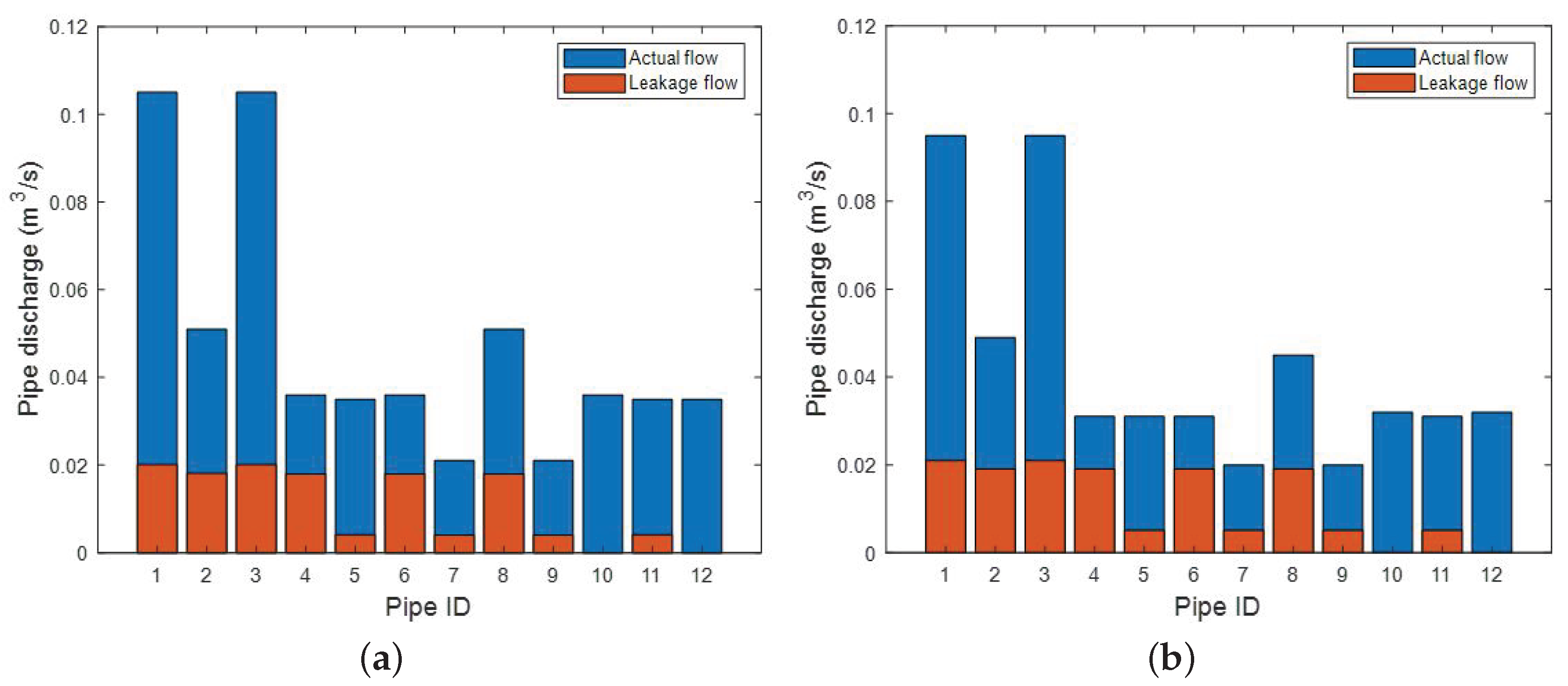
By analyzing the profile of the pipe discharge and the pipe leakage flow for both scenarios as presented in Figure 3, it is obvious in Figure 3a that the leakage flow in some pipes, for example, pipes 1, 3, 5, 7, 9, 10, 11, and 12, is much lower when compared to their corresponding pipe discharge. Moreover, for pipes 2, 4, 6, and 8, the leakage flow is almost half of their corresponding discharge, as can be seen in Figure 3a. In Figure 3b for the PDM case, and in a similar manner to the result presented in Figure 3a, it is observed that the level of the leakage flow in pipes 1, 3, 5, 7, 9, 10, 11, and 12 is much lower compared to their corresponding actual pipe discharge. However, for pipe 4 and 6, the leakage flow is more than half of their corresponding discharge.
Comparing both figures, for the PDM case in Figure 3b, the level of the leakage flow in all the pipes is slightly higher than those in Figure 3a for the DDM analysis. As discussed earlier, the reason for this is the relatively high pressure head status observed in the PDM when compared to the DDM case for this network. In addition, no leakage flow is noticed in pipes 10 and 12 for both cases. These pipes (i.e., pipes 10 and 12) are connected to node 9 which is characterized by a negative pressure.
The total network flows at the pipe and node levels are compared for both scenarios, the results are shown in Figure 4. As observed in the DDM analysis (Figure 4a), the leakage flow at the pipe level is almost 25% of the total pipe discharge. However, for the PDM case in Figure 4b, about 33% is lost as a result of leakage. Considering the node level, about 33% of the total demand is lost as a result of leakage for the DDM analysis (Figure 4a) and around 37% for the PDM analysis (Figure 4b). From this analysis, it may be observed that the total network leakage level for the PDM case is higher than that of the DDM case. As explained in the other figures, the reason for this is the relatively high pressure head status observed in the PDM when compared to the DDM case for this network.
The above investigations are also considered for a much larger network designed for an industrial area in Southern Italy. Figure 1b relays the schematics of the WSN used for this numerical example (network 2). The network is a real planned water supply network designed for an industrial area in the town of Apulia (a city in Southern Italy). The network consists of 34 pipes interconnected between 24 nodes. The pipes have varying lengths and diameters, which range from 158.2 m to 955.7 m and 100 mm to 368 mm, respectively. As observed in Figure 1b, water is supplied from node 24 at a head of 36.45 m. Furthermore, the demand at the junction nodes varies between 7.575 L/s to 17.034 L/s. The Hazen–Williams model is used for the head loss estimation. The Hazen–Williams coefficient for all the pipes is equal to 150. The data relevant to this network may be found in [34]. For this network, the PDM analysis was executed by setting the minimum and the service pressure heads to 10 m and 30 m, respectively.
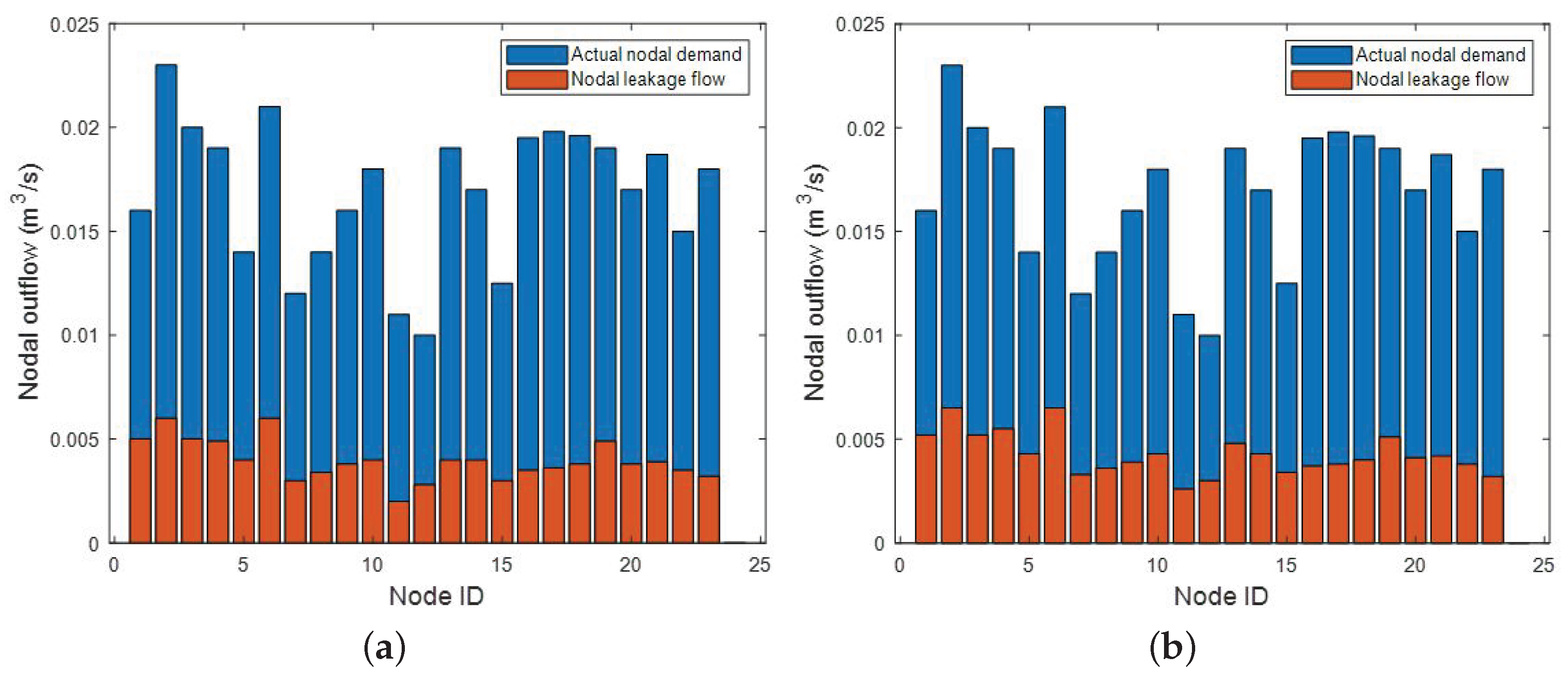
Figure 5 relays the profile of the nodal leakage flow with regard to the particular demand for this case study (network 2); Figure 5a for the DDM analysis and Figure 5 for the PDM analysis. In both scenarios and in a similar manner to the results presented in Figure 2, it is observed that the level of the leakage flow at the node is much lower compared to the demand. Additionally, for both scenarios, the leakage and the demand at the node follows similar patterns. More importantly, the level of the leakage flow for the PDM analysis is slightly higher than that of the DDM analysis. This is due to the relatively high pressure status observed in the PDM when compared to the DDM case for this network.
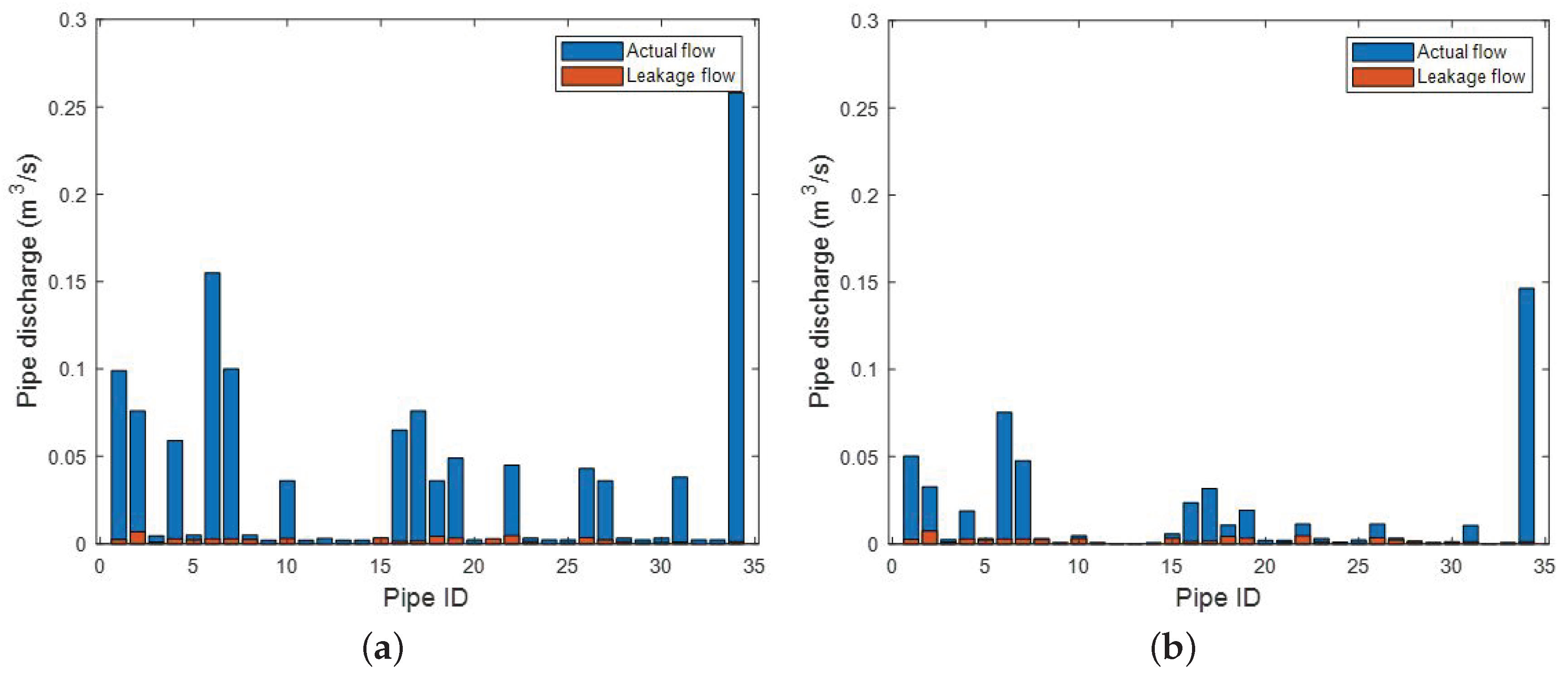
In terms of the pipe discharge and the pipe leakage flow for both scenarios as presented in Figure 6, for obvious reasons, the actual flow in each pipe for the PDM analysis (Figure 6b) is relatively low compared to that of the DDM analysis (Figure 6a). Depending on the network boundary conditions, when PDM conditions are used, the required demand at the nodes is generally lower than (or at the most, equal to) the DDM case. Therefore, the estimated required flow in the pipes is expected to decrease for the PDM case. In a situation where the supplied network boundary conditions are such that the demand at the nodes is satisfied, the flow in the pipes for the PDM case is expected to be equal to that of the DDM case. Moreover, the level of the leakage flow for both scenarios is almost the same and is close to zero. However, this is slightly higher for the PDM case as may be noticed in pipe 2 and pipe 22. Thus, for both simulation scenarios, almost all the pipes are characterized by nearly zero leakage flows. The same pattern is observed for both simulation scenarios.
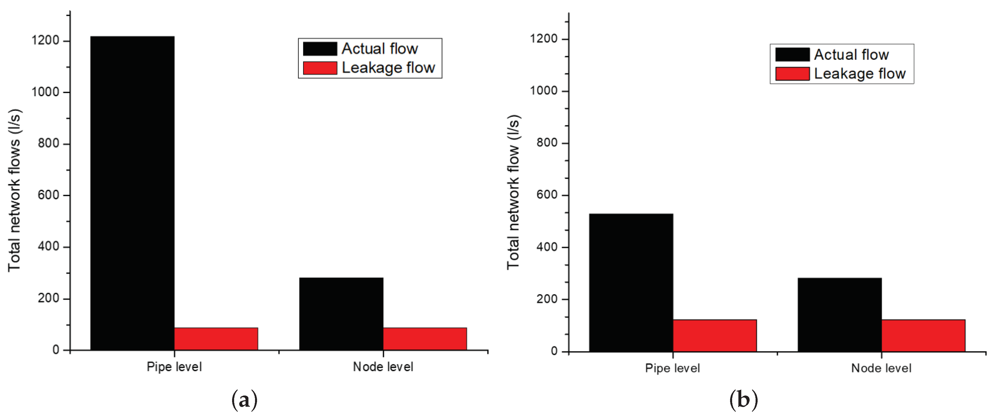
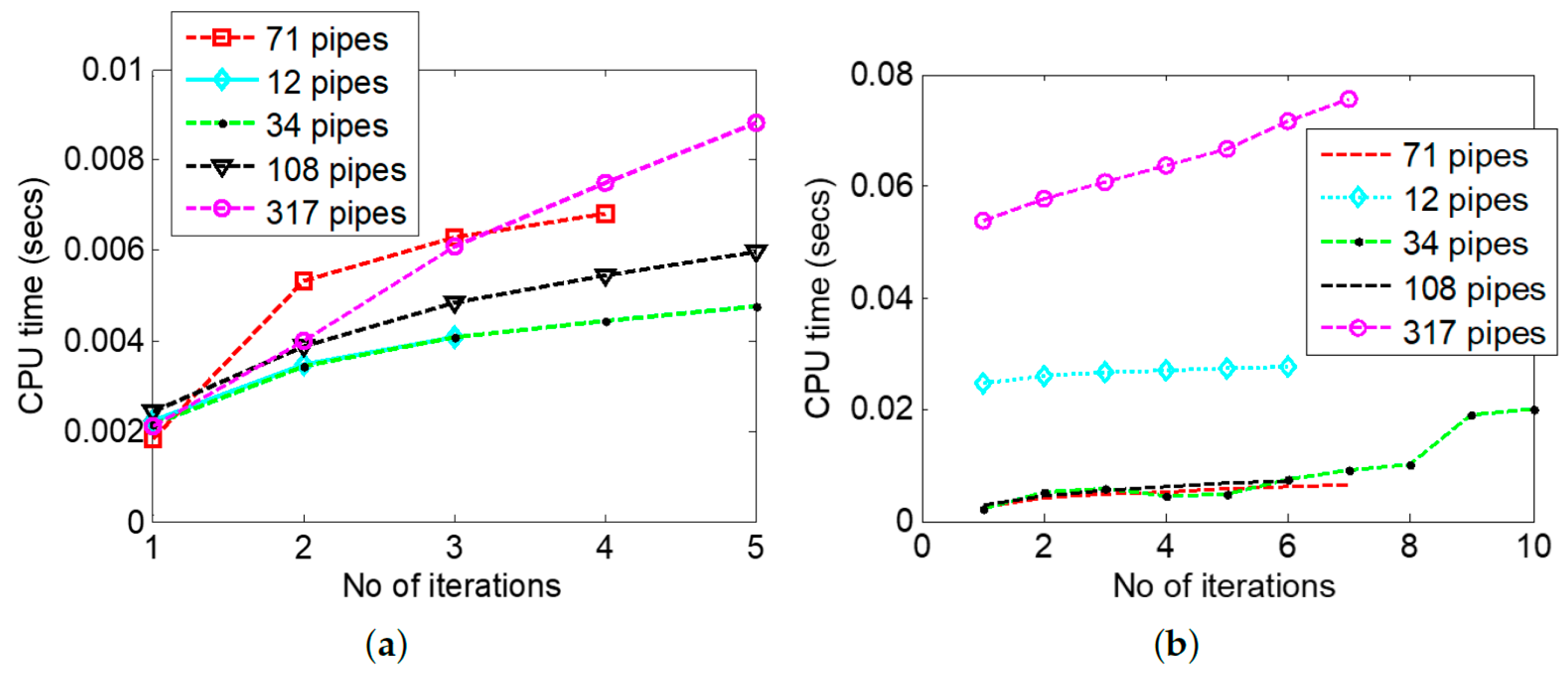
In Figure 7, the overall network leakage at the node and pipe level with respect to the actual pipe discharge and the nodal demand for both DDM (Figure 7a) and PDM (Figure 7b) is compared. Considering the pipe level, almost 8% of the total flow is lost through leakage for the DDM analysis, as is shown in Figure 7a, while nearly 23% of the flow is lost through leakage when the PDM analysis in Figure 7b is considered. Moreover, the node level analysis revealed that about 33% of the total network demand is lost through leakage when the DDM analysis is considered (Figure 7a) while about 45% is lost for the PDM analysis (Figure 7b). Figure 8 shows the computational solution time of the results obtained for the case study WSNs and three other WSNs; the network characteristics are shown in Table 1, considering both simulation scenarios, when computed on the MATLAB R2013a software on a hp EliteBook 8560p computer with a 6 GB RAM and 64-bit operating system. These results show that the DDM case (Figure 8a) is faster to compute than the PDM case (Figure 8b).
It is interesting to note that the computational time difference for both scenarios is not much, thus, the computational efficiency of the PDM is considered favorable because of its usefulness in portraying the behavior of WSNs. It is also noticed that these depend on the network data and the network boundary conditions (i.e., in the supplied and for each network for the PDM case). More importantly, the objective of this work was to investigate and analyze the influence a PDD function has on background leakage estimate in order to improve the leakage detection algorithm developed in Adedeji et al. [21]. Comparing the proposed PDM solution to other PDM solutions in the literature will be addressed in the future research papers.
4. Conclusions
This study appraises the effect of a pressure-dependent demand on the background leakage estimation utilizing two WSNs as numerical cases. The results presented demonstrate that the reliance of the nodal demand on the available pressure head at the node impacts the magnitude of the background leakage flow at the pipe and node level. While the DDM analysis is faster to compute as compared to the PDM case, it is important to note that the computational efficiency of the PDM is favorable considering its usefulness in portraying the real behavior of water supply networks. It is envisaged that this analysis may be fundamental for background leakage estimation for networks operating under pressure-deficient conditions. Finally, it is important to note that the leakage results for the PDM case rely upon the available pressure head at the node. If the current pressure head at the node is adequate to completely fulfill consumer demand, the upper boundary condition of the PDD function is satisfied, and subsequently, the magnitude of the leakage flow at the node and pipe level, for PDM analysis, will be the same as that of the conventional demand-driven modeling analysis. This is also subject to the size of the network as well as the network boundary conditions.
Author Contributions
The work is part of the Doctorate degree of K.B.A. which was discussed with his supervisors. K.B.A. formulated the problem and drafted the manuscript. Y.H. assisted with improvements in the mathematical formulations. The manuscript was reviewed by Y.H. while A.M.A.-M. also advised on some improvements.
Funding
This research work is supported by the Tshwane University of Technology and the Council for Scientific and Industrial Research, Pretoria, South Africa under the smart network initiatives.
Acknowledgments
This research work was supported by Tshwane University of Technology, Pretoria and the Council for Scientific and Industrial Research (CSIR), Pretoria, South Africa.
Conflicts of Interest
The authors declare no conflict of interest.
Appendix A. Continuation of the PDM with Background Leakage Model Derivation
Starting from Equation (4), the matrices and are derived from the network topological incidence matrix A expressed as
It should be noted that background leakage flow runs continuously along the length of a pipe. Therefore, if the vector of the leakage flow rate along the pipe is denoted by , then may be expressed [26] as
Thus, the vector may be computed using the topological incidence matrix as
where is an empirical constant relating to background leakage parameter of the jth pipe, is the length of the jth pipe, denotes the leakage-pressure exponent reported to be equivalent to 1.18 for background leakage [26], and is the pressure head vector in pipe j computed as the mean of the pressure head values at its end nodes.
From Equation (6), the Jacobian matrix J of the function in (6) may be expressed as
where is a diagonal matrix of size and is a diagonal matrix of size .
In (A6), N is expressed as , a diagonal matrix of dimensions . The elements of N are the partial derivatives of the head loss relation (excluding minor loss due to valves) with respect to q. Likewise, is a diagonal matrix of dimensions whose elements are the partial derivatives of the pressure-dependent demand (PDD) function in (2) with respect to the nodal pressure head. For a node i, may be expressed as
In addition, in Equation (A6), is a diagonal matrix of size whose elements are the derivatives of the nodal leakage vector . The allocation of the leakage flow is such that half of the total leakage flow from the pipe occurs at the end nodes. Thus, the elements of are computed from derivatives of with respect to . The matrix for a node i may be expressed as
where
Therefore, when Newton–Raphson method is applied to Equation (6) at each iteration “k” the application of the NR method gives
Multiplying both sides of (A11) by , it is possible to write
Therefore, the estimate of the nodal head may be obtained by substituting in (A12) into (A13) and replacing by a matrix B as
Moreover, the estimate of the flow in each pipe may be extracted from Equation (A11) as
References
- Adedeji, K.B.; Hamam, Y.; Abe, B.T.; Abu-Mahfouz, A.M. Towards achieving a reliable leakage detection and localization algorithm for application in water piping networks: An overview. IEEE Access 2017, 5, 20272–20285. [Google Scholar] [CrossRef]
- Wu, Z.; Farley, M.; Turtle, D.; Kapelan, Z.; Boxall, J.; Mounce, S.; Dahasahasra, S.; Mulay, M.; Kleiner, Y. Water Loss Reduction, 1st ed.; Bentley Institute Press: Exton, PA, USA, 2011. [Google Scholar]
- Hindi, K.S.; Hamam, Y. Locating pressure control elements for leakage minimisation in water supply network: An optimisation model. Eng. Optim. 1991, 17, 281–291. [Google Scholar] [CrossRef]
- Hindi, K.S.; Hamam, Y. Pressure control for leakage minimisation, in water distribution networks, Part 1, Single period models. Int. J. Syst. Sci. 1991, 22, 1573–1585. [Google Scholar] [CrossRef]
- Hindi, K.S.; Hamam, Y. Pressure control for leakage minimisation, in water distribution networks, Part 2, Multi-period models. Int. J. Syst. Sci. 1991, 22, 1587–1598. [Google Scholar] [CrossRef]
- Page, P.R.; Abu-Mahfouz, A.M.; Yoyo, S. Real-time adjustment of pressure to demand in water distribution systems: Parameter-less P-controller algorithm. Procedia Eng. 2016, 154, 391–397. [Google Scholar] [CrossRef]
- Page, P.R.; Abu-Mahfouz, A.M.; Yoyo, S. Parameter-less remote real-time control for the adjustment of pressure in water distribution systems. J. Water Res. Plan. Manag. 2017, 143, 04017050. [Google Scholar] [CrossRef]
- Page, P.R.; Abu-Mahfouz, A.M.; Mothetha, M.L. Pressure management of water distribution systems via the remote real-time control of variable speed pumps. J. Water Res. Plan. Manag. 2017, 143, 04017045. [Google Scholar] [CrossRef]
- Adedeji, K.B.; Hamam, Y.; Abe, B.T.; Abu-Mahfouz, A.M. Pressure management strategies for water loss reduction in large-scale water piping networks: A review. In Advances in Hydroinformatics; Gourbesville, P., Cunge, J., Caignaert, G., Eds.; Springer: Singapore, 2018; pp. 465–480. [Google Scholar]
- Sechi, G.M.; Zucca, R. A cost-simulation approach to finding economic optimality in leakage reduction for complex supply systems. Water Resour. Manag. 2017, 31, 4601–4615. [Google Scholar] [CrossRef]
- Azevedo, B.B.; Saurin, T.A. Losses in water distribution systems: A complexity theory perspective. Water Resour. Manag. 2018, 32, 2919–2936. [Google Scholar] [CrossRef]
- Araujo, L.S.; Ramos, H.; Coelho, S.T. Pressure control for leakage minimisation in water distribution systems management. Water Resour. Manag. 2006, 20, 133–149. [Google Scholar] [CrossRef]
- Farah, E.; Shahrour, I. Leakage detection using smart water system: Combination of water balance and automated minimum night flow. Water Resour. Manag. 2017, 31, 4821–4833. [Google Scholar] [CrossRef]
- Leu, S.S.; Bui, Q.N. Leak prediction model for water distribution networks created using a Bayesian network learning approach. Water Resour. Manag. 2016, 30, 2719–2733. [Google Scholar] [CrossRef]
- Page, P.R.; Abu-Mahfouz, A.M.; Piller, O.; Mothetha, M.; Osman, M.S. Robustness of parameter-less remote real-time pressure control in water distribution systems. In Advances in Hydroinformatics; Gourbesville, P., Cunge, J., Caignaert, G., Eds.; Springer: Singapore, 2018; pp. 449–463. [Google Scholar]
- Abu-Mahfouz, A.M.; Hamam, Y.; Page, P.R.; Adedeji, K.B.; Anele, A.O.; Todini, E. Real-time dynamic hydraulic model of water distribution networks. Water 2019, 11, 470. [Google Scholar] [CrossRef]
- Todini, E. A more realistic approach to the extended period simulation of water distribution networks. In Advances in Water Supply Management; Swets and Zeitlinger Publishers: Lisse, The Netherlands, 2003. [Google Scholar]
- Braun, M.; Piller, O.; Deuerlein, J.; Mortazavi, I. Limitations of demand-and pressure-driven modelling for large deficient networks. Drink. Water Eng. Sci. 2017, 10, 93–98. [Google Scholar] [CrossRef]
- Giustolisi, O.; Berardi, L.; Laucelli, D.; Savic, D.; Walski, T.; Brunone, B. Battle of back- ground leakage assessment for water networks at WDSA conference 2014. Procedia Eng. 2014, 89, 4–12. [Google Scholar] [CrossRef]
- Covelli, C.; Cimorelli, L.; Cozzolino, L.; Della Morte, R.; Pianese, D. Reduction in water losses in water distribution systems using pressure reduction valves. Water Sci. Technol. Water Supply 2016, 16, 1033–1045. [Google Scholar] [CrossRef] [Green Version]
- Adedeji, K.B.; Hamam, Y.; Abe, B.T.; Abu-Mahfouz, A.M. Leakage detection and estimation algorithm for loss reduction in water piping networks. Water 2017, 9, 773. [Google Scholar] [CrossRef]
- Bhave, P.R. Node flow analysis distribution systems. Transp. Eng. J. ASCE 1981, 107, 457–467. [Google Scholar]
- Wagner, J.M.; Shamir, U.; Marks, D.H. Water distribution reliability: Simulation methods. J. Water Res. Plan. Manag. 1988, 114, 276–294. [Google Scholar] [CrossRef]
- Chandapillai, J. Realistic simulation of water distribution system. J. Transp. Eng. 1991, 117, 258–263. [Google Scholar] [CrossRef]
- Wu, Z.Y.; Wang, R.H.; Walski, T.M.; Yang, S.Y.; Bowdler, D.; Baggett, C.C. Extended global-gradient algorithm for pressure-dependent water distribution analysis. J. Water Res. Plan. Manag. 2009, 135, 13–22. [Google Scholar] [CrossRef]
- Germanopoulos, G. A technical note in the inclusion of pressure dependent demand and leakage terms in water supply network models. Civ. Eng. Syst. 1985, 2, 171–179. [Google Scholar] [CrossRef]
- Reddy, L.S.; Elango, K. Analysis of water distribution networks with head-dependent outlets. Civ. Eng. Syst. 1989, 6, 102–110. [Google Scholar] [CrossRef]
- Tanyimboh, T.; Templeman, A. A new nodal outflow function for water distribution networks. In Proceedings of the 4th International Conference on Engineering Computational Technology, Lisbon, Portugal, 7–9 September 2004; Civil Comp Press: Stirling, UK, 2004. [Google Scholar]
- Tabesh, M.; Shirzad, A.; Arefkhani, V.; Mani, A. A comparative study between the modified and available demand driven based models for head driven analysis of water distribution networks. Urban Water J. 2014, 11, 221–230. [Google Scholar] [CrossRef]
- Anonymous. Fire Suppression Rating Schedule, 6th ed.; Insurance Services Office: New York, NY, USA, 1980. [Google Scholar]
- Twort, A.; Law, F.; Crowley, F.; Ratnayaka, D. Water Supply, 4th ed.; Edward Arnold: London, UK, 1994. [Google Scholar]
- Adedeji, K.B. Development of a Leakage Detection and Localisation Technique for Real-Time Applications in Water Distribution Networks. Ph.D. Thesis, Department of Electrical Engineering, Tshwane University of Technology, Pretoria, South Africa, 2018. [Google Scholar]
- Hamam, Y.; Brameller, A. Hybrid method for the solution of piping network. Proc. IEE 1971, 118, 1607–1612. [Google Scholar] [CrossRef]
- Giustolisi, O.; Todini, E. Pipe hydraulic resistance correction in WDN analysis. Urban Water J. 2009, 6, 39–52. [Google Scholar] [CrossRef]
Figure 1.
The schematics of the case study networks used for the numerical examples: (a) network 1; (b) network 2.
Figure 1.
The schematics of the case study networks used for the numerical examples: (a) network 1; (b) network 2.

Figure 2.
Nodal demand vs. the leakage flow for each node for the case study network 1: (a) demand-driven modeling (DDM) analysis; (b) pressure-driven modeling (PDM) analysis.
Figure 2.
Nodal demand vs. the leakage flow for each node for the case study network 1: (a) demand-driven modeling (DDM) analysis; (b) pressure-driven modeling (PDM) analysis.

Figure 3.
The pipe discharge and the leakage flow in each pipe for the case study network 1: (a) DDM analysis; (b) PDM analysis.
Figure 3.
The pipe discharge and the leakage flow in each pipe for the case study network 1: (a) DDM analysis; (b) PDM analysis.

Figure 4.
Total network leakage flow with respect to the nodal demand and pipe discharges for the case study network 1: (a) DDM analysis; (b) PDM analysis.
Figure 4.
Total network leakage flow with respect to the nodal demand and pipe discharges for the case study network 1: (a) DDM analysis; (b) PDM analysis.

Figure 5.
Nodal demand vs. the leakage outflow for each node for the case study network 2: (a) DDM analysis; (b) PDM analysis.
Figure 5.
Nodal demand vs. the leakage outflow for each node for the case study network 2: (a) DDM analysis; (b) PDM analysis.

Figure 6.
The pipe discharge and the leakage flow for the case study network 2: (a) DDM analysis; (b) PDM analysis.
Figure 6.
The pipe discharge and the leakage flow for the case study network 2: (a) DDM analysis; (b) PDM analysis.

Figure 7.
Total network leakage flow with respect to the nodal demands and pipe discharges for the case study network 2: (a) DDM analysis; (b) PDM analysis.
Figure 7.
Total network leakage flow with respect to the nodal demands and pipe discharges for the case study network 2: (a) DDM analysis; (b) PDM analysis.

Figure 8.
Comparison of the solution time for the case study networks: (a) CPU time for the DDM case; (b) CPU time for the PDM case.
Figure 8.
Comparison of the solution time for the case study networks: (a) CPU time for the DDM case; (b) CPU time for the PDM case.


Table 1.
Characteristics of the case study networks used for the performance test.
| Network ID | Head-Loss Model Used | (m) | (m) | Total Required Demand (L/s) | ||||
|---|---|---|---|---|---|---|---|---|
| N1 | 12 | 9 | 8 | 1 | HW | 0 | 10 | 208.1 |
| N2 | 34 | 24 | 23 | 1 | HW | 10 | 30 | 282 |
| N3 | 71 | 46 | 45 | 1 | HW | 5 | 20 | 88.82 |
| N4 | 108 | 70 | 67 | 3 | HW | 5 | 90 | 535 |
| N5 | 317 | 272 | 268 | 4 | HW | 5 | 80 | 406.94 |
Note: HW: Hazen-Williams.
© 2019 by the authors. Licensee MDPI, Basel, Switzerland. This article is an open access article distributed under the terms and conditions of the Creative Commons Attribution (CC BY) license (http://creativecommons.org/licenses/by/4.0/).
Share and Cite
MDPI and ACS Style
Adedeji, K.B.; Hamam, Y.; Abu-Mahfouz, A.M. Impact of Pressure-Driven Demand on Background Leakage Estimation in Water Supply Networks. Water 2019, 11, 1600. https://doi.org/10.3390/w11081600
AMA Style
Adedeji KB, Hamam Y, Abu-Mahfouz AM. Impact of Pressure-Driven Demand on Background Leakage Estimation in Water Supply Networks. Water. 2019; 11(8):1600. https://doi.org/10.3390/w11081600
Chicago/Turabian StyleAdedeji, Kazeem B., Yskandar Hamam, and Adnan M. Abu-Mahfouz. 2019. "Impact of Pressure-Driven Demand on Background Leakage Estimation in Water Supply Networks" Water 11, no. 8: 1600. https://doi.org/10.3390/w11081600
Note that from the first issue of 2016, this journal uses article numbers instead of page numbers. See further details here.