Hydropower from the Alpine Cryosphere in the Era of Climate Change: The Case of the Sabbione Storage Plant in Italy


Department of Civil and Environmental Engineering DICA, Politecnico di Milano, L. da Vinci 32, 20133 Milano, Italy
*
Author to whom correspondence should be addressed.
Water 2019, 11(8), 1599; https://doi.org/10.3390/w11081599
Submission received: 3 July 2019
/
Revised: 30 July 2019
/
Accepted: 30 July 2019
/
Published: 1 August 2019
(This article belongs to the Section Hydrology)
Abstract
:Greenhouse gas reduction policies will have to rely as much as possible upon renewable, clean energy sources. Hydropower is a very good candidate, since it is the only renewable energy source whose production can be adapted to demand, and still has a large exploitation margin, especially in developing countries. However, in Europe the contribution of hydropower from the cold water in the mountain areas is at stake under rapid cryospheric down wasting under global warming. Italian Alps are no exception, with a large share of hydropower depending upon cryospheric water. We study here climate change impact on the iconic Sabbione (Hosandorn) glacier, in the Piemonte region of Italy, and the homonymous reservoir, which collects water from ice melt. Sabbione storage plant has operated since 1953 and it was, until recently, the highest altitude dam of Europe at 2460 m asl, and the former second largest dam of the Alps with 44 Mm3. We use two models, namely Poly-Hydro and Poly-Power, to assess (i) present hydrological budget and components (i.e., ice/snow melt, rainfall), and (ii) hydropower production under optimal reservoirs’ management, respectively. We then project forward hydrological cycle including Sabbione glacier’s fate, under properly downscaled climate change scenarios (three General Circulation Models, three Representative Concentration Pathways, nine scenarios overall) from IPCC until 2100, and we assess future potential for hydropower production under the reservoir’s re-operation. Mean annual discharge during 2000–2017 is estimated at 0.90 m3 s−1, with ice melt contribution of ca. 11.5%, and ice cover as measured by remote sensing changing from 4.23 km2 in 2000 to 2.94 km2 in 2017 (−30%). Mean hydropower production during 2005–2017 is estimated as 46.6 GWh. At the end of the century ice covered area would be largely depleted (0–0.37 km2), and ice melt contribution would drop largely over the century (0%–10%, 5% on average at half century, and null in practice at the end of century). Therefore, decreased ice cover, and uncertain patterns of changing precipitation, would combine to modify the future stream fluxes (−22% to −3%, −10% on average at half century, and −28% to 1%, average −13%, at the end of century). Power production, driven by seasonal demand and water availability, would change (decrease) in the future (−27% to −8%, −15% on average at half century, and −32% to −5%, −16% at the end of century). Our results demonstrate potential for decrease of cold water in this area, paradigmatic of the present state of hydropower in the Alps, and subsequent considerable hydropower losses under climate change, and claim for adaptation measures therein.
1. Introduction
Greenhouse gas reduction policies will have to rely upon renewable, clean energy sources. Hydropower is a largely clean source of energy, and yet it depends upon water availability, and proper management [1]. In Europe, and worldwide, hydropower comes largely from cold water, originating from ice/snow melt in the mountain areas, and is often exploited via storage, and subsequent (optimal) operation [2], also under a multi-purpose perspective [3,4]. Such contribution is however at stake, in terms of timing and amount, under the recent rapid cryospheric down wasting in response to global warming [2,5], and in general under climate driven hydrological changes [5]. The Alps of Italy, and Europe are no exception, with their large share of water depending upon the cryospheric areas [6,7,8,9], and at significant risk under climate change (e.g., [10]).
Global glacier retreat started past the Little Ice Age [11], occurring between XIV and XIX centuries, when the temperature in the Northern Hemisphere was lower on average by −0.6 °C [12]. Indeed, glacier retreat is taken as major evidence of climate change, and Alpine glaciers have been particularly affected by temperature rise [13,14,15,16,17]. While in the XX century the global average temperature increased by +0.9 °C [18] above the pre-industrial era, in the Alps an increase of 1.4 °C was estimated [19]. The Swiss Glacier Inventory, dating back until 1850, made it possible to estimate the Alpine glacierized area variation over the last 150 years or so. According to [20], the Alpine ice covered area passed from 4474 km2 in 1850 to 2272 km2, in 2000 with a loss of −49%. In the Italian Alps, the first accurate Glacier Inventory dates back to 1962, with an estimate of 509 km2 of total area. Such value increased to 609 km2 in the inventory of 1984 (possibly due to different monitoring systems, and noise in the previous assessment), and subsequently dropped to 368 km2 in 2015 [21].
Mountain glaciers’ depletion worldwide may affect many fields, i.e., mountain tourism [22], sea-level rising [23,24], hydrological regimes [7,25,26], and, especially for high altitude reservoirs, hydropower production [27]. The latter is affected by glaciers’ retirement, and by modified dynamics of seasonal snow cover [2,5,9].
To unravel the complex nexus between cryospheric water and hydrological cycle, climate, and hydropower potential, one needs tools able to (i) accurately mimic the cryospheric processes, and components of hydrological flows [28], including snow accumulation, snow/ice melting, glacier’s mass budget and dynamics, (ii) evaluate potential hydrological variations under prospective climate change scenarios, and (iii) assess the effects upon hydropower potential even under complex water management in storage plants (e.g., [27]). In this work, we assess the effects of the present and potential future climate upon the Sabbione reservoir, located in the Formazza valley, in the Piemonte region of Italy. Particularly, we estimate the impact of climate change upon retirement of the Sabbione glacier’s, and the hydrological cycle of the basin, and we study subsequent changes in reservoir management and hydropower production.
The artificial 1.2 km2 Sabbione lake (2460 m asl), formed by the Sabbione dam (64 m high, 279 m wide, 44 Mm3 of maximum storage), collects water from the 14.5 km2 Sabbione basin, nesting the Sabbione/Hosandorn glacier (2.7 km2), whose rapid retreat is a concern for the ENEL (Ente Nazionale per l’ELettricità) company of Italy, the plant’s owner, since it may modify future production and revenues. A steel pipe from the plant’s toe delivers water to a power plant placed ca. 640 m downstream, then releasing water in the Morasco lake (1815 m asl), which is artificially regulated for power production.
We used here the Poly-Hydro model, well suited for simulation of hydrological cycle in cryospheric areas [29] to implement hydrological modelling during a calibration period 2000–2017, and then we pursued projections until 2100. We used here climate outputs from three general circulation models (plus downscaling) under three RCPs. We then used the Poly-Power model, which takes inputs of discharges, and energy price (present, and projected), to optimally manage the reservoir, aiming at maximizing revenues, now and over the century [27].
The manuscript is organized as follows. In the section “Case study” we present the area of interest, and main characteristics of hydrology, and plant’s operation. In the section, “Data Base” we describe the data base used here for setup, and validation of the models. In “Methods,” we depict the main traits of our models. In the section “Results,” we display the projected modified hydrological cycle, and hydropower production. In the section “Discussion,” we benchmark our findings against recent literature, we comment on dependability of the results against uncertain projections of future climate, and provide limitations, and outlooks. We then provide a “Conclusions” section, where we summarize our study.
2. Case Study
Val Formazza valley covers north of Piemonte region, in the Lepontine Alps of Italy. Toce River collects water of the valley, subsequently delivering to Lago Maggiore lake. Toce river originates from Cascata del Toce (Frua) waterfall (143 m), regulated by Morasco dam at 1815 m asl near Riale (Charbäch). The Sabbione dam (ca. 2460 m asl, 64 m tall) was built between 1949 and 1953 by Edison Spa Company, upstream of Morasco dam, close to the Swiss border.
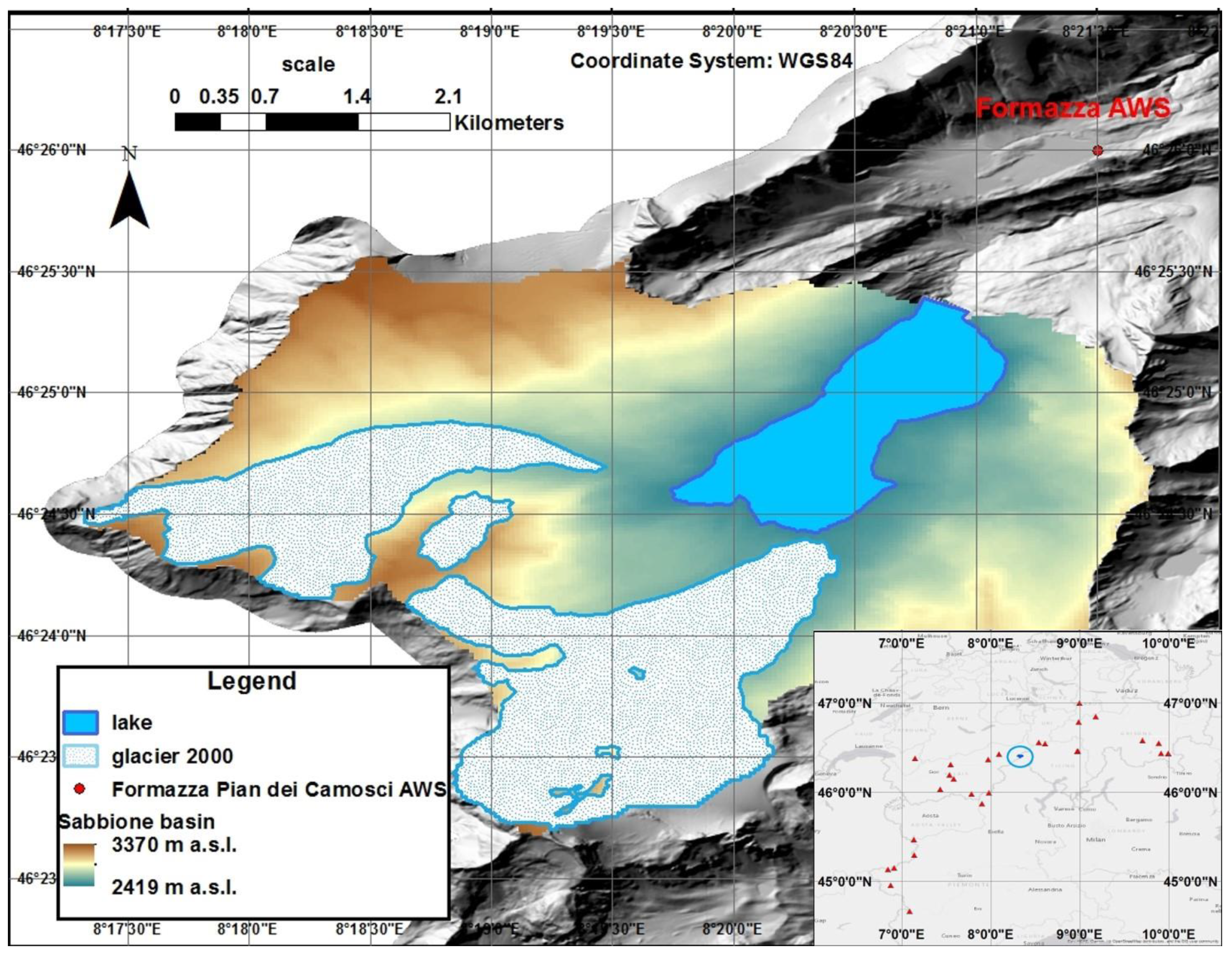
The catchment of the dam, with area 14.5 km2, has 2.7 km2 (ca. 19%) covered by ice (November 2017), and bare rocks mostly (Figure 1). The basin includes three mountain summits, the highest being Blinnehorn, at 3374 m asl, so the total altitude jump in the basin is ca. 914 m.
A 985 m long pipe takes water from the lake to a downstream power plant (ca. 645 m vertical jump), made of two Pelton turbines, on the shore of Morasco lake (1815 m asl, slightly varying for regulation).
Average temperature registered by an automatic weather station (AWS), located at Pian dei Camosci at 2453 m asl, during 2000–2017 is 0.0 °C (annual mean maximum/minimum temperature, being 4.4/−3.8 °C). The coldest month is January, with −7.3 °C on average, and the hottest is July with 8.0 °C on average. Mean annual rainfall is 874 mm (with the least rain in January, 4.7 mm on average, and largest in August, 161 mm on average), and mean snow precipitation, measured as snow water equivalent SWE, is 987 mm (minimum of 1 mm in July, and maximum of 192 in November on average).
The oldest data available for Sabbione glacier dates back to 1898, i.e., in the “Geologische Karte der Simplon-Gruppe,” displaying a glacier surface reaching to the present dam position. In 1954 when the dam was built however, the glacier was already split into three parts (Northern, Central, and Southern), as visible in Figure 1. The artificial Sabbione lake partially drowned the southern part of the glacier, further accelerating shrinking. By the 80s the glacier emerged by the lake, which in turn reached its present capacity, Vres = 44 Mm3. Mazza and Mercalli [30] estimated a 1600 m retirement of the glacier’s front during 1885–1987, with a loss of volume of −50% or so. In the last 30 years, the glacier continued to shrink (e.g., [31]), reaching an area of 2.7 km2 (2017), with several rock outcrops that interrupt the glacier’s continuity.
3. Data Base
3.1. Poly-Hydro Model Setup (2000–2017)
To sketch the local topography for set up of the Poly-Hydro model we used a 25 m digital terrain model DTM, built using LIDAR technology within the HELI-DEM project [32]. The nearest automatic weather station (AWS) available is Formazza Pian dei Camosci, property of Agenzia Regionale Protezione dell’Ambiente ARPA (46°25′60″ N, 8°21′30.00″ E, 2453 m asl), about 1400 m away from the dam (Table 1). The AWS station provides data on temperature, rainfall, and snow depth, or new daily snow, the latter to be converted into SWE using estimates of snow density as from daily minimum temperature (e.g., [33,34]). We further used data from 29 other temperature stations in the Western Alps, to estimate the monthly vertical lapse rate of temperature, to extrapolate temperature at single cells in the model as a function of altitude (see Table 2). We searched for vertical gradient in total precipitation using data from stations at high altitude with both pluviometer and snow-gauge, but by the small number of stations with these characteristics (we found only nine stations in the Western Alps) no visible vertical lapse rate of precipitation was detected. Therefore, also considering the relatively small size of the catchment, we assumed constant precipitation in space (however separated into snow/rain according to local temperature).
Whenever data from the AWS station at Pian dei Camosci were not available, we provided interpolation using data from Formazza Bruggi AWS station (46°20′52.00″ N, 8°35′44.00″ E, 1226 m asl), ca. 11 km away from the dam.
Theoretical, topographically corrected clear sky radiation in Sabbione catchment was calculated, and further corrected for cloudiness via a clear sky index (CSI), i.e., the ratio between observed and theoretical radiation. This was calculated using daily measured radiation data at Grimsel Hospiz (46°34’18’’ N, 08°19’60’’ E, 1980 m asl), in Switzerland, ca. 16 km away from the dam. The so corrected radiation estimates were subsequently used to assess ice/snow melting via a mixed degree day model (e.g., [7]). We subsequently assessed average monthly values of CSI index during clear/rainy days, to be applied for assessment of corrected radiation for future climate projections (see also [35]).
3.2. Glacier’s Cover Dynamics (2000–2017)
To track glacier evolution during the calibration period (2000–2017), we used several orthophotos, and satellite images. The initial condition for glacier cover was taken from interpretation of an ortophoto from November 1999. Model validation was subsequently pursued using orthophotos in 2007, 2012, 2015, and a satellite image in 2017 (see Table 3). The glacier’s outline was pursued manually, with a specific focus upon the potential presence of seasonal snow cover, and debris coverage (however negligible here), as necessary in glaciers’ cover definition (e.g., [9,36]). The images were mostly taken in late summer, so normally little snow was available. During summer 2011, a research group composed by IMAGEO srl, and the Italian Meteorological Society SMI pursued a campaign on the Southern Sabbione glacier, installed four ablation stakes, that were subsequently monitored every year (in September), until summer 2016. These stakes recorded an average yearly loss of ice thickness of about 200 cm on the glacier. Since there were no records of ice flow dynamics (i.e., flow velocity), when setting up the ice flow module of Poly-Hydro model, we used ice flow parameters from measures in a well monitored Alpine glacier [7]. Rough GPR (Ground Penetrating Radar) estimates of ice thickness during 2011 in some sections of the Sabbione glacier were kindly made available by IMAGEO company (personal communication, 11 June 2018), and we used such estimates for ice flow validation.
3.3. Hydropower Production and Price
No specific data for hydropower production or reservoir management of Sabbione dam (like daily storage level or electricity production) were made available from ENEL that we know of. Long term average information of hydropower production was available anyway [37]. Mean year power production was equal to 45.4 GWh [37]. Maximum turbines’ discharge is 8.1 m3 s−1 (two Pelton turbines). However, we assumed that only one turbine operates at a time, given that even during the summer monthly peak (i.e., 2.23 m3 s−1 in July), discharge is well below 4 m3 s−1. Energy prices after energy liberalization in Italy (2005–2017) are continuously made available by Gestore dei Mercati Energetici (GME) S.p.A., an Italian authority with the mission of promoting the development of a national competitive electricity system, according to the criteria of neutrality, transparency, and objectivity. We used historical energy price from GME to simulate reservoir management that maximizes the revenue from electricity production.
3.4. Climate Projections (2018–2100)
To project forward hydrology, and thence hydropower production in the Sabbione reservoir, we used mean temperature and precipitation scenarios from CMIP5 of the IPCC (Intergovernmental Panel on Climate Change, CMIP5) [38], namely ECHAM6 (European Centre HAmburg Model, version 6) [39], CCSM4 (Community Climate System Model, version 4), and EC-Earth (European Consortium Earth system model, version 2.3) [40]. We used these GCMs in past studies (e.g., [25]), and they displayed acceptable capacity of representing the climate of the area. We used three Representative Concentration Pathways (RCP) that are scenarios of greenhouse gas concentration trajectories. We used RCP 2.6, a most optimistic scenario, with +1 °C estimated increase of mean global temperature at the end of XXI century, RCP 4.5 (+2.2 °C) and RCP 8.5 (+3.7 °C). Due to the low spatial resolution of these models (100–200 km), statistical downscaling of precipitation and temperature was necessary (see [29,41]), which we set up against ground data (AWS Formazza) during 2000–2017. By doing so, we obtained nine scenarios of climate, which we could use as inputs to the Poly-Hydro model for projecting forward hydrological cycle, and energy demand/price dynamics in the Sabbione reservoir.
4. Methods
4.1. Ice Flow Modelling and Mass Balance
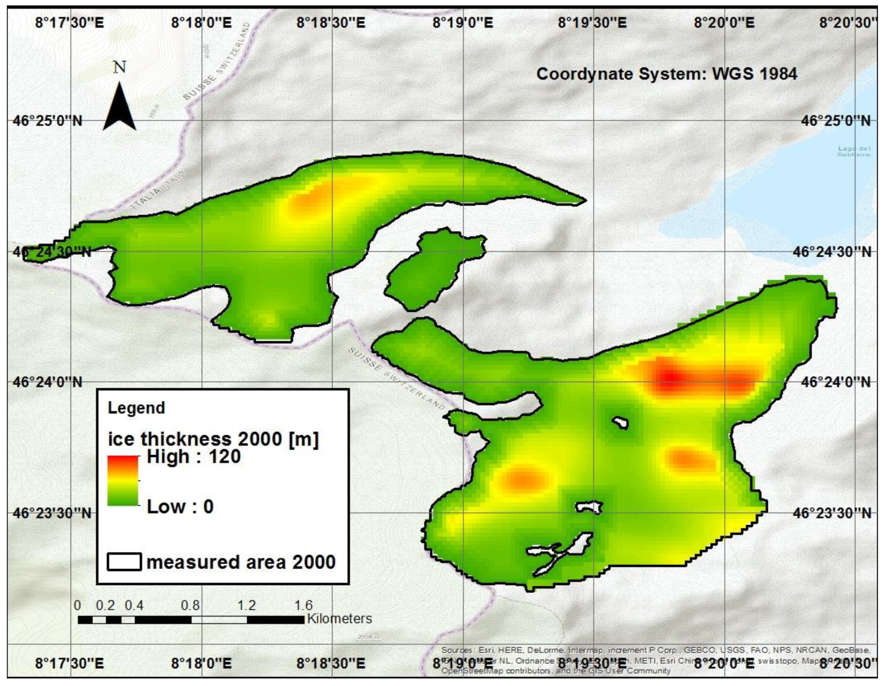
The Poly-Hydro model uses the ice-flow module Poly-Ice, which adopts a simplified force-balance scheme, to picture flow velocity, proportional to (basal) glaciers shear stress according to Glen’s law (see full description e.g., in [7,42]). Such module requires an input of ice thickness for each cell of the basin, here in year 2000 when the simulation starts. Given that we were able to measure glacier’s perimeter from orthophotos as reported, we could use the glaciers’ shape, and local altitude from DEM, to estimate glacier thickness against local slope, and basal shear stress τb (Pa). The latter can be in turn estimated, e.g., from glacier’s altitude jump ΔH (the difference between maximum and minimum glacier’s altitude), using an empirical formula by Haeberli and Hoelzle [43]:
τb = 0.005 + 1.598∆H − 0.435∆H2 if ∆H < 1.6 km
τb = 1.5 if ∆H > 1.6 km
τb = 1.5 if ∆H > 1.6 km
Once τb is calculated for each of the three different glacier’s bodies (Figure 1), we can evaluate ice thickness hice with the equilibrium equation by Oerlemans [44]:
where ρice is ice density (917 kg m−3), g is gravity, sinα is the sinus of local slope of the bedrock, regarding this last value, since DEM allows us to evaluate only ice slope, we had to impose an iterative cycle where we evaluated bedrock slope subtracting hice (initially found using ice slope data) to DEM and then using these values to re-evaluate hice until convergence. To account for low thickness in the terminus and along the borders, we applied within the first 100 m (four cells) from glacier’s edges a linear (with distance from the edges) reduction factor (0.2–1) for hice.
Poly-Ice pursues daily glacier’s mass balance depending upon snow, and ice accumulation/melting. To model snow/ice melting we used a mixed (temperature + radiation) degree day approach (e.g., [7])
Mice,snow = TMFice,snow × (T − TThresh) + RMFice,snow × G × CSI × (1 − αice,snow)
if T > TThresh
Mice,snow = 0 if T < TThresh
if T > TThresh
Mice,snow = 0 if T < TThresh
Therein Mice,snow (mm d−1) is the melting of either ice or snow within a cell, T is air temperature [°C], TMFice,snow (mm d−1 C−1), and RMFice,snow (mm d−1 W−1 m−2) are the temperature and radiation melting factors, for either ice or snow, αice,snow (-) is the ice/snow albedo (here taken as 0.3/0.7 as an average value from observed data upon Alpine glaciers, see Soncini et al. [7]). TThresh is an air temperature threshold (0 °C here as from data analysis). G (W m−2) is the theoretical clear sky, topographically corrected global radiation, and CSI (-) clear sky index as explained above. First, we calibrated snow melt factors using snow depth measures at the AWS Formazza (2009–2017). As the objective performance indicator we chose Nash-Sutcliffe coefficient NSE, using as the control variable the ground snow depth, estimated by the model, and measured in the AWS Formazza.
We then applied the so obtained melt factors at the glacier scale to simulate snow, and ice melt using Poly-Hydro during 2000–2017. During this exercise, we often observed in Poly-Hydro outputs an unlikely long persistence of snow pack on the glacier (i.e., snow cover would persist across the whole summer season). As a result, Poly-Hydro would provide little to null ice melting (given that ice melts normally starts after snow thaw) in large spots upon the glacier. However, using the data from our four ablation stakes (2011–2016), we could verify considerable ice melt in those years (200 cm per year on average). Accordingly, we had to increase slightly the melt factors, keeping as a criterion to have modeled snow depth consistently with observation (NSE > 0.85), and so as to obtain a more likely snow cover pattern. Once estimated for the calibration period the day with no snow cover, we could calibrate ice melt factors, maximizing NSE using as observed data the measured ice melt at ablation stakes. In practice for ice melting however, we found a negligible effect of radiation (i.e., RMFice was 0 in practice), with much larger effect of temperature.
4.2. Hydrological Model
Poly-Hydro is a semi-distributed, physically based, glacio-hydrological model, already used and validated in several studies [4,7,45]. Poly-Hydro is able to reproduce different components of the hydrological cycle, and cryospheric processes. Here we synthetically depict the model, already well described elsewhere [7,35]. Poly-Hydro tracks soil water balance for each cell at a daily scale, from inputs of precipitation (rainfall), and snow/ice melt, and outputs of actual evapotranspiration, surface and sub-surface discharge. Precipitation is partitioned (rain/snow) using a threshold temperature (here 0 °C) of mean daily temperature. Potential evapotranspiration (also used for lake evaporation) ETP is evaluated using Hargreaves–Samani equation [46]. We evaluated sub-surface discharge as a function of terrain permeability and water content; surface discharge is given by excess of water with respect to saturation level. Due to the small size of our basin (14.5 km2), and mainly rocky nature of the soil, we made the simplifying hypothesis that the daily runoff reaches the outlet in the same day, so no flow routing was necessary.
4.3. Hydropower Production Model
We used Poly-Power to investigate hydropower production under the reasonable assumption of reservoir management aimed at maximizing yearly profit, as expected from hydropower companies. Poly-Power is a physically based model, usable to constrain production against objective functions. Here we report a brief description of Poly-Power, already depicted elsewhere [28]. Poly-Power uses as as input (i) energy price in 6 h scale (in order to catch price variation within a day) (ii) reservoir’s input flows (from Poly-Hydro), (iii) pool-level/volume curve of the reservoir (here to simplify computation we considered constant level with volume, since the change in head given by level oscillation in the dam is a small fraction of total jump, i.e., ±15 m, i.e., ±2.3% of the 645 topographic jump), and in general geometry of the plant, and provides as an output optimal power production (where optimality here is given by maximum revenue), in line with proper constraints (reservoir between min and max level, i.e., 2430–2460 m asl, operated discharge between 0 and max, 4.05 m3 s−1). Since the model works in yearly batches, maximizing revenue from year to year, one needs to avoid emptying of the lake at the end of every year, resulting from an attempt of maximizing the yearly revenue.
A penalty function was thus considered. This consists of the revenue given by the sale of the energy produced with a change in volume between the last day and the first day of the year (a positive sign is considered if this change is positive and vice versa). The efficiency of energy production is considered constant, which is likely given the balance between the efficiency of the Pelton turbine(s), generally maximum at the largest discharges, and the high loss of energy in the pipe with high discharges.
4.4. Hydrological and Hydropower Projections Until 2100
Using the nine scenarios (three GCMs, three RCPs) of climate produced by downscaling of IPCC scenarios as reported, we fed the projected climate inputs into the Poly-Hydro model, for projecting forward hydrological cycle, and glacier dynamics in the Sabbione area. We subsequently used the so obtained hydrological scenarios to evaluate future hydropower production.
Future energy demand/price has been projected using the model in Bombelli [47]. This model first takes into account projections of gross domestic product GDP by OECD (Organisation for Economic Co-operation and Development), climate change (temperature) modelled using IPCC scenarios, uncertainty in the form of random factors to assess variability in energy demand, and the day of the year (week days, holidays, etc.). Dependence from the mean daily temperature is described in terms of the power needed for heating and cooling when the temperature deviates (below, or above) from proper thresholds [48]. Subsequently, energy price is estimated as a function of temperature, volatility, and the day of the year.
The model was tuned against available energy price data (2005–2017) made available by GME as reported, with acceptable results [47].
Once future hydrology, and energy price were estimated, we could use Poly-Power to maximize future revenues, and to evaluate the corresponding energy production, against the present one. We focused upon one recent control period CR, 2005–2017 (13 years, when energy prices were available), and then considered two reference future periods (15 years), namely P1 2045–2059, and P2 2086–2100.
5. Results
5.1. Modelling of Sabbione Glacier
In Table 4 we report tuning of the Poly-Hydro model parameters (mostly melt factors for snow and ice), and goodness of fit statistics when applicable. In Figure 2 we report the initial (year 2000) condition of Sabbione glaciers’ ice covered area ICA as set in the Poly-Hydro model based on an orthophoto of November 1999, as reported. In Figure 3 we can see subsequent ICA simulation from Poly-Hydro in the years 2007, 2012, 2015, and 2017, benchmarked against their estimated counterparts, from various sources as reported, and against initial ICA in 2000. In Table 5, we report the validation scores of the modeled ICA for the four years above.
Generally speaking, the model seems to acceptably depict glacier dynamics, and especially ice retire, with slightly decreasing overall accuracy over time. In 2007, there is a quite good matching between the modeled and observed ICA in the South part, while the model slightly over-estimated retirement in the center, and North area. Overall, the ICA is well matched, and the percentage error is Err% = 0%. In 2012, Poly-Hydro provides slightly overestimated ice loss (−4% ICA), visible both in North and South ice bodies.
In 2015 and 2017 conversely, glaciers’ down wasting seems to accelerate, and Poly-Hydro simulation is lagging in this sense, especially in the South fraction. In 2017 the estimated glacier area is 2.9 km2, while the measured ICA is 2.7 km2 (about +8% overestimate). Since the model is capable of depicting changes of ice cover (−31% from 2000–2017 for the model, −36% from measures), we could use it to estimate change in water volume stored by the Sabbione glacier, that passed from 122.6 × 10⁶ m3 in 2000 to 53.7 × 10⁶ m3 in 2017 with a reduction of −56% ca.
5.2. Stream Flows and Hydropower Production
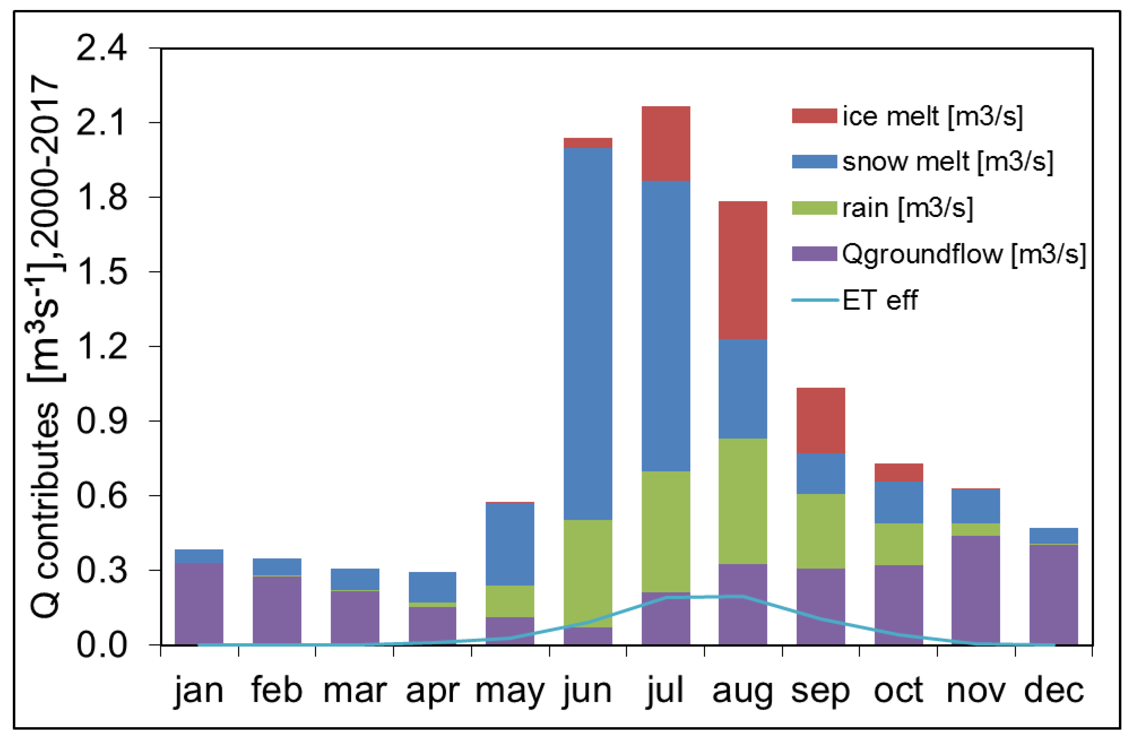
Average estimated monthly flows from the Sabbione catchment are given in Figure 4, evapotranspiration is also reported, which can be considered as a negative flow component since it subtracts water to the basin. The yearly mean discharge was estimated as 0.90 m3 s−1, with monthly maxima of ca. 2.23 m3 s−1 on average in July, and minima nearby 0.30 m3 s−1 in April. The maximum annual discharge computed is in 2015 with 1.24 m3 s−1, while minimum in 2000 with 0.60 m3 s−1, where snow accumulated during the previous year was not considered. Snow melt contributes, on average, 39% of the total discharge (maximum 73% in June, minimum 14% in December), while ice melt covers 11% on average (maximum 32% in August, minimum is 0%, December to May). Yearly evapotranspiration counts for 124 mm of water on average (almost 90% of it occurring between June and September), that is about 7% of total precipitation.
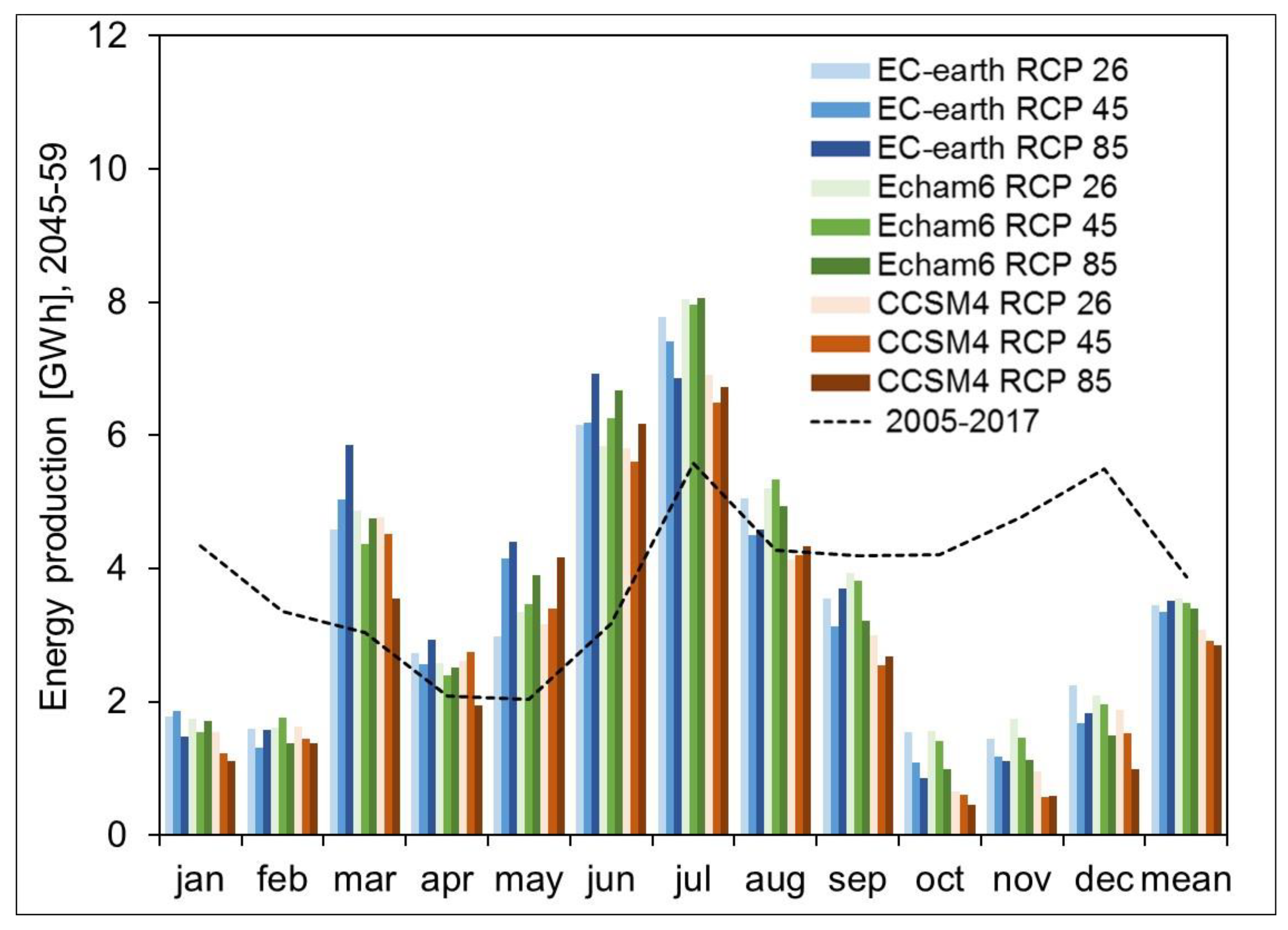
In Figure 5 we report monthly (and yearly mean) hydropower production, referred to the CR period (2005–2017, after 2004 energy market liberalization). Our mean estimated yearly production is E[Ep] = 46.6 GWh. This value is slightly bigger (+3%) than the 45.4 GWh data as provided by ENEL data base as reported, and yet seemingly acceptable.
Accordingly, and in spite of poor data availability related to reservoir management, and production, the Poly-Hydro + Poly-Power model seems to provide an acceptable depiction of the hydropower production process here. Power production Ep is least in spring (likely in the wake of the low flow winter, with emptying of the reservoir), and largest between August and December (after large accumulation in the wake of summer thaw).
5.3. Future Hydro-Climatology
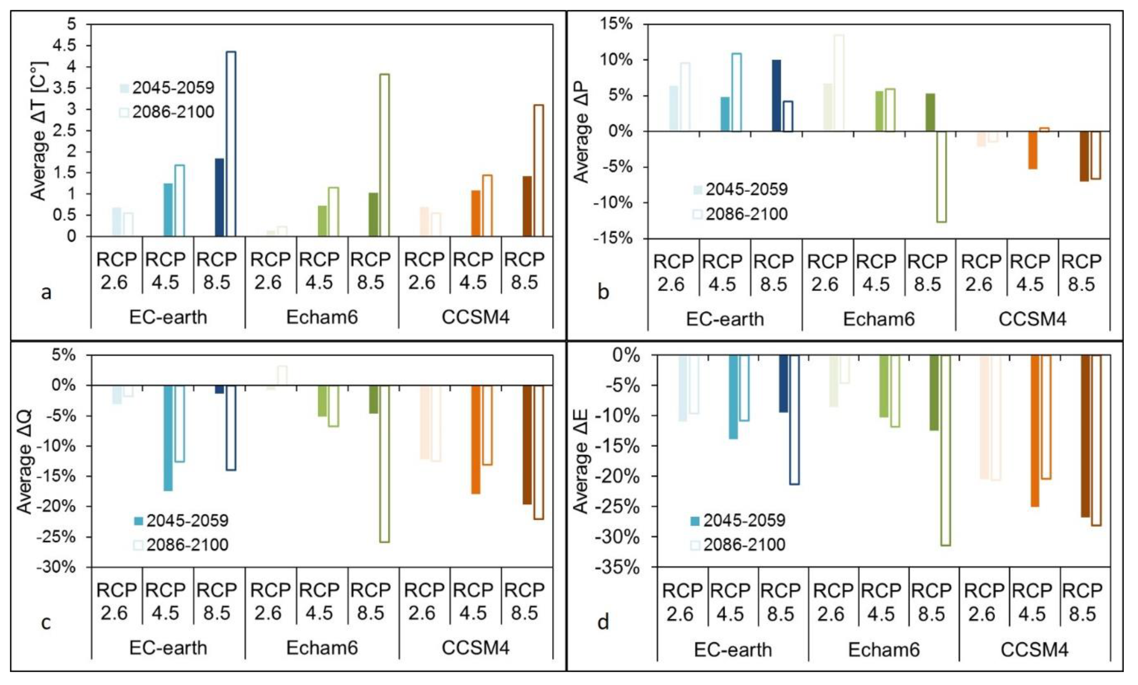
In Figure 5 and Figure 6 we provide the relative changes of mean air temperature (at Formazza AWS station) as projected within our nine scenarios against the CR for the periods P1 and P2. Visibly, temperature always increases over the century, albeit with chances of reduction late in the century under RCP2.6 (EC-Earth, and CCSM4), as a result of potentially intense mitigation as set out under this RCP. In the most extreme RCP8.5, changes of temperature may reach up to +4.5 °C increase against CR.
Precipitation changes are reported similarly in Figure 7. Here, more variability is seen, typical of projections over a century in the Alpine area as here (e.g., [8]). A worst case scenario (−13%) is seen during P2 under RCP8.5 of ECHAM model, with instead mostly increasing precipitation under EC-Earth scenarios. The CCSM4 model displays mostly decreasing precipitation, however.
In Figure 7, the corresponding scenario of catchment flows are given. Indeed, mostly negative changes of the yearly flow are projected, unless for RCP2.6 of ECHAM6, and mostly P2 would be the driest period.
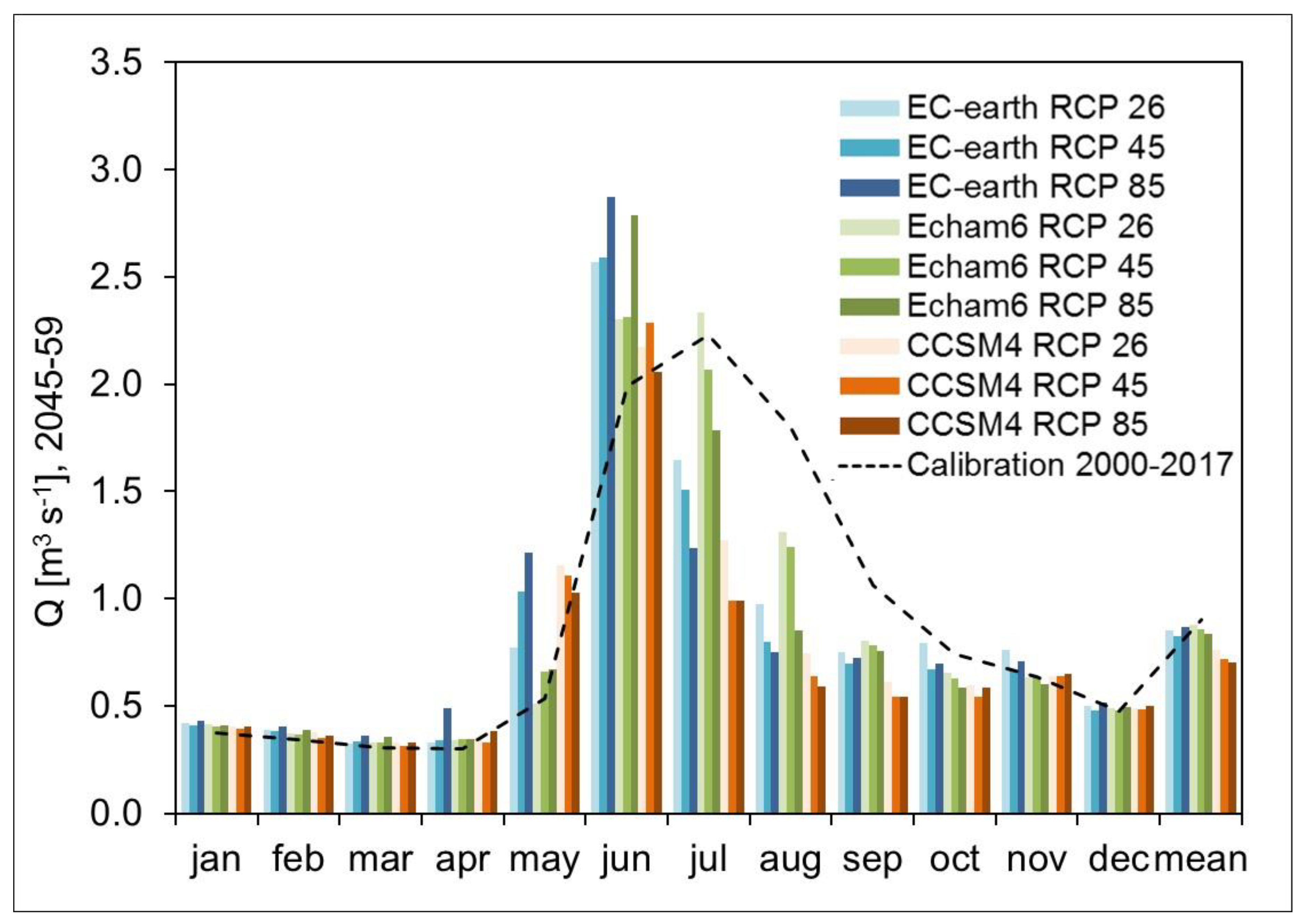
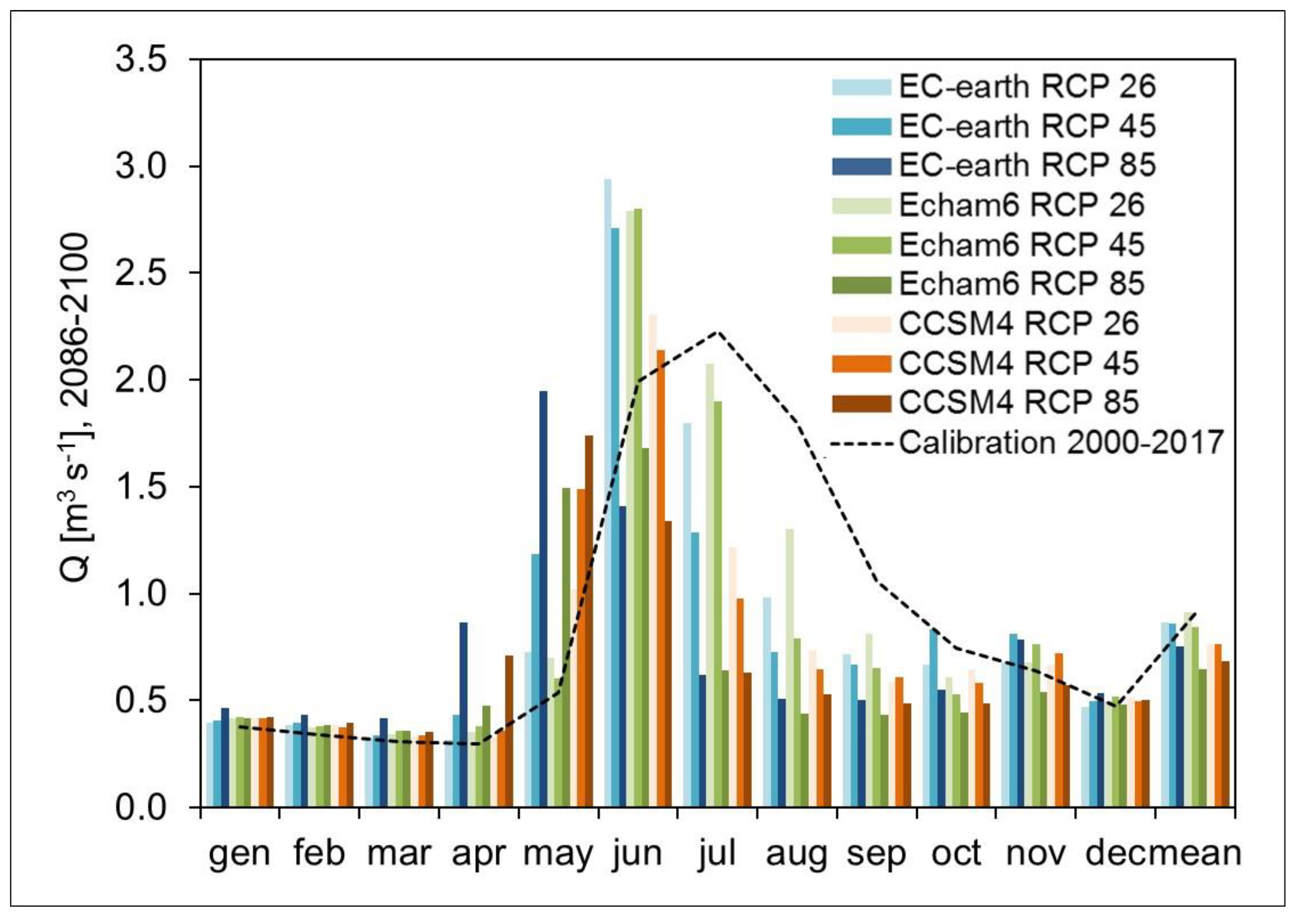
In Figure 8 and Figure 9, the projected monthly (and yearly mean) dynamics of stream flows is given. Visibly, mean projected flows would become much smaller than now during the wettest season (July–October). A visible increase would clearly occur in spring (May–June), but not enough to make up for summer lack of water.
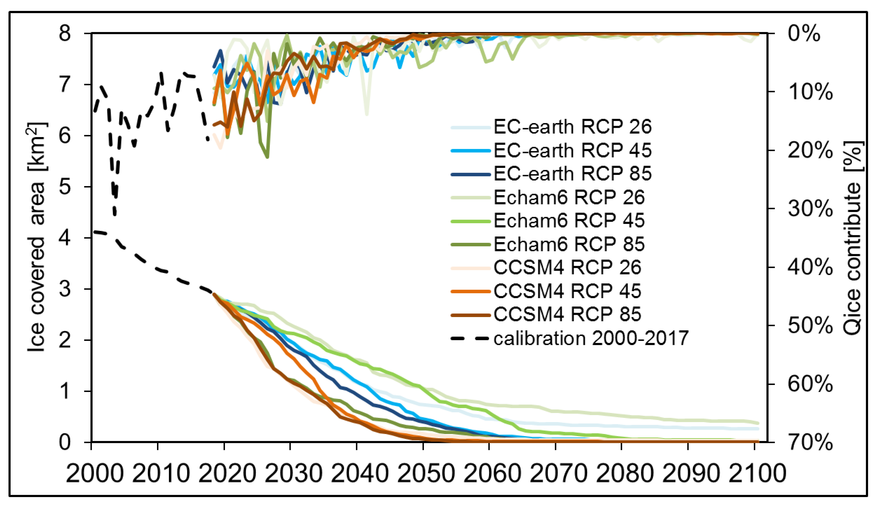
In Figure 10 we report the projected ice covered area ICA over the century until 2100, together with the mean yearly share of stream flows from ice melt Qice. Visibly, large reduction of the ICA would occur under all of our nine scenarios over the century, with complete down wasting at half century or slightly later under RCP8.5 of all GCMs.
Ice flow contribution reaches nowadays about 11% on average, with the peak close to 30% or so in some years (i.e., 2003). In the future as seen, such contribution will reach lower and lower values, until disappearance in practice at 2060 or so. Accordingly, one could expect that reduced ice melt contribution will result in reduced stream flows overall. Considering P1 and P2, in Figure 7 one has a decrease ΔQ of −22% to −3%, with −10% on average in P1, and −28% to +1%, and −13% on average during P2.
The only scenario with an increase in stream flow is RCP2.6 of ECHAM6 during P2, which displays in Figure 7 a large expected increase of precipitation ΔP (+13%), that is the only condition to have stream flows equal to, or larger than, present levels.
5.4. Future Hydropower Production
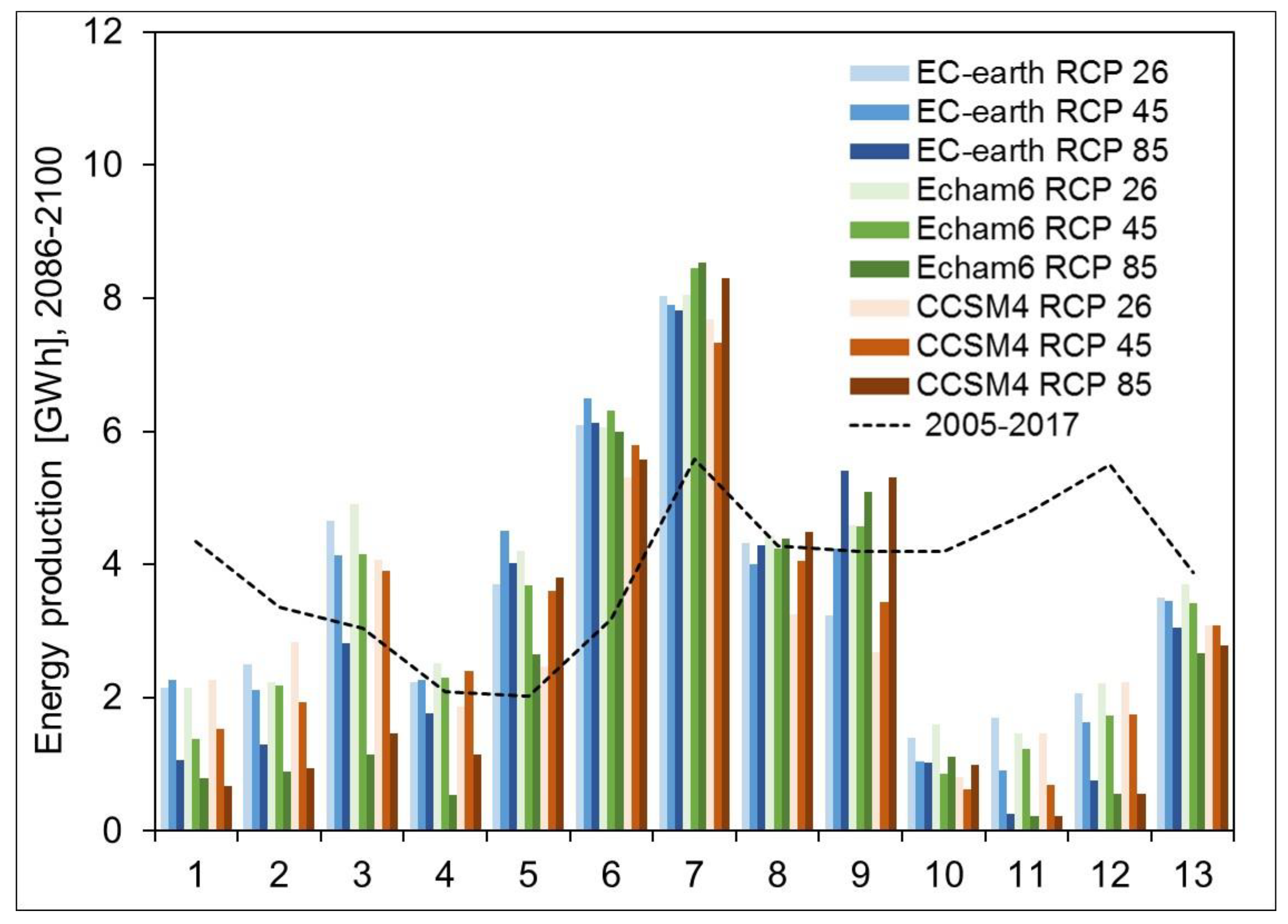
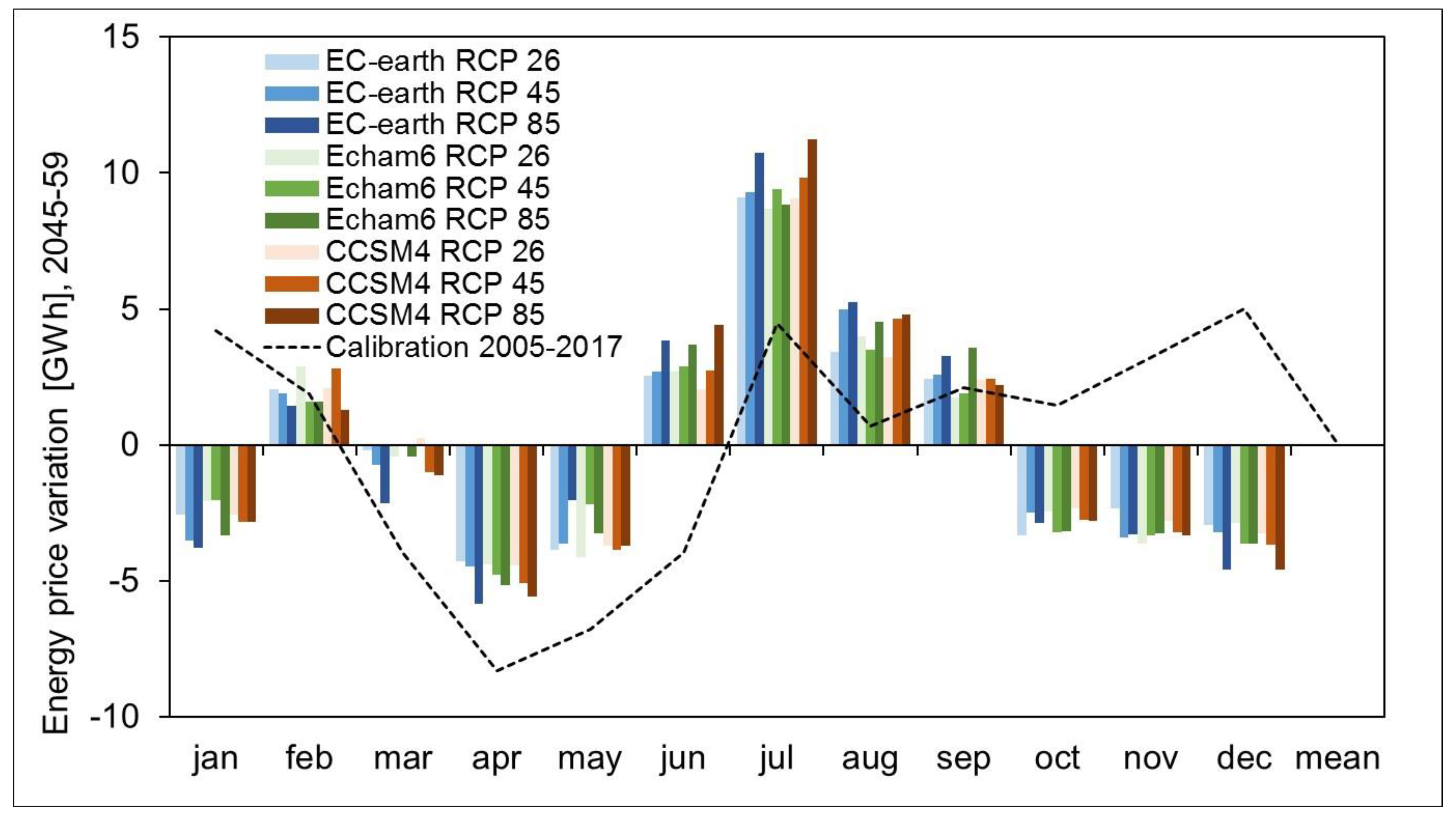
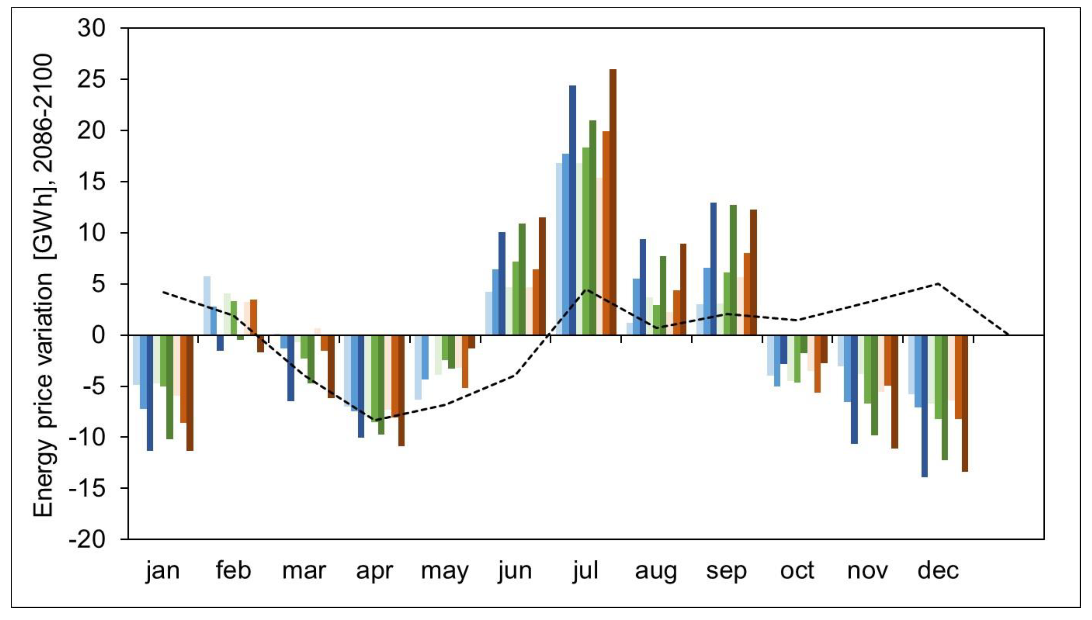
Projected changes of hydropower production ΔEp at the yearly scale are given in Figure 7, and in Figure 5 and Figure 6 the projected monthly (and yearly mean) energy production is given. In Figure 11 and Figure 12 we display the projected monthly energy price relative to annual mean, as calculated by Poly-Power for the two reference periods, against the CR scenario. This provides an insight of the relative price (value) of hydropower energy during different months, and of the seasonal shifting of the price dynamics.
Clearly from Figure 7 ΔEp is negative under every scenario, i.e., year-round hydropower production would decrease considerably until the end of the century. Worst case scenarios are under RCP8.5 at P2, somewhat consistently with the expectedly decreased water availability in those period/RCPs as from Figure 7. Figure 5 and Figure 6 demonstrate seasonal monthly dynamics of Ep.
Visibly, there is much more variability in energy production, with large decrease during fall and winter (OND, and JF), and increase in late winter, spring, and early summer (M, AMJ, JA).
Looking at Figure 11 and Figure 12, one generally finds a consistent response of energy production dynamics to energy price (and demand).
From October to January, energy demand for heating decreases due to temperature rising (Figure 6), so (relative) energy price in Figure 11 and Figure 12 decreases. February remains under all scenarios the coldest month in the year (not shown for shortness), so a slight increase of the relative price in this month remains, similarly to now, and yet much lower than in the warm season. Production in fall and winter is therefore lower than in the Control Run period.
During spring and early summer in P1, conversely temperature increases, with larger cooling need than in the CR period, and therefore higher energy price from March to August, and subsequently production increases therein.
Then, in late summer (September), production would again decrease slightly in response to a decrease of price.
During P2, a similar pattern would be seen, with some differences however. In March and April production would be reduced, especially under the RCP8.5 scenarios (Figure 6), because relative energy price would decrease (Figure 12). From June to September energy price would still increase, especially under RCP8.5, and production would increase against CR, and even against P1 in September. In August however, production during P2 would be lower than during P1 on average. From Figure 8 and Figure 9, during Summer (JAS), and especially August, stream flows Q to the reservoir would be considerably smaller than now, most notably under RCP8.5 in P2. Accordingly, during August, and partly September, production would be lower than now in the P2 period, due to lack of seasonal water therein.
Over the century, late spring and summer would display an increasingly earlier peak of stream flows (Figure 8 and Figure 9) as due to seasonal snow melt, with a decrease in flows in August, and September, much wetter nowadays given large decrease of ice melt. Energy price dynamics also shift visibly towards earlier, with the largest increase of cooling energy demand in the hottest months of June and July, and peaking flows in these months apparently would sustain energy demand. During August and September (P2), however, also increasing temperature and energy prices would demand larger cooling energy than now, but in this case low flows would not allow consistent production, in spite of regulation.
6. Discussion
6.1. Recent Cryospheric Dynamics of High Altitude Alpine Catchment
Our findings concerning the retreat of Sabbione glacier and stream flow components can be benchmarked against some recent results in the Italian Alps.
Bocchiola et al. [25] studied the evolution of glaciers (2006–2009) within the Pantano catchment of the Adamello group (2.14 km2 ICA), in Lombardia, at an altitude close to that of the Sabbione glacier (2480–3222 m asl in Adamello vs. 2460–3474 m asl at Sabbione). Ice melt estimated therein (2006–2008) was −2.2 m of water equivalent per year (m w.e.year−1).
Mandrone Glacier (about 12 km2), also in Adamello group, was recently estimated to have wasted (1995–2009) about −1.4 m w.e.year−1, with largest melt in 2003 (−3.05 m w.e.year−1, [49]).
Grossi et al. [49] also provided mass balance of the Presena glacier (0.95 km2, 1995–2009) in Lombardia, namely −1.50 m w.e.year−1 (and −3.09 m w.e.year−1 in 2008), and of the Caresèr Glacier (about 2.8 km2), with –1.69 m w.e.year−1 (and −3.32 m w.e.year−1 in 2003).
Soncini et al. [7] estimated −1.06 m w.e.year−1 during 1996–2008 for the Dosdè glacier in Alta Valtellina valley of Italy. During 2009–2014, the mass loss of Dosdè glacier increased to −1.53 m w.e.year−1.
Garavaglia et al. [50] investigated the past (1929–2007) and prospective (until 2100) mass balance of the Forni Glacier (about 11.4 km2, the largest valley glacier in Italy). They found a mean mass balance (1981–2007) of −0.97 m w.e.year−1, with the largest loss ever in 2003, i.e., −6.36 m w.e.year−1.
Diolaiuti [51], Cannone et al. [52], and more recently Smiraglia (2015, personal communication in 2018) evaluated mass balance of the Sforzellina Glacier (nearby Forni glacier, 0.36 km2, see D’Agata et al. [53]). For Sforzellina Glacier (0.36 km2) several studies confirmed a negative mass balance [51,52], Smiraglia and Diolaiuti [21] evaluated, during 1987–2014, −1.06 m w.e.year−1, that increased to −1.19 m w.e.year−1 for 2000–2014, with the largest loss in 2003 (−2.20 m w.e.year−1).
During our period of calibration (2000–2017), we estimated an average loss of −1.47 m w.e.year−1.
The magnitude of cryospheric processes depends upon ice cover, normally increasing with ice cover, and they can be main drivers of discharge like Sabbione basin here, with 28% ice cover (2000).
During 2000–2017 we estimated that yearly snow and ice shares of snow and ice were 39% and 11%, respectively, i.e., half of yearly flows are due to cryospheric processes, the other half being rainfall. Snow melt contribution reaches its peak in June with a 73% share, and then it represents 52% and 23% of stream flows in July and August. Ice melt is relevant from July to September, with a peak of share in August (32%).
Bocchiola et al. [25] showed that about 50% of the spring and summer flows (2006–2009) in Pantano catchment derived from ice and snow ablation, with ice melt share variable during the season, but in the order of 35% yearly (and ICA 19.5% of the catchment).
Soncini et al. [7], during May–September (2009–2014), estimated for Dosdè catchment (mean altitude 2858 m asl, 17 km2) that snow melt covers about 47% of stream flows, and ice melt covers 10% (ICA, 11% of the area).
According to Aili et al. [8], in Curlo catchment (89 km2, mean altitude 2740 m asl, ICA 6 km2), snow melt contribution to flow during spring and summer (1981–2017) is about 47%, while ice melt share in summer is about 6%. Our results are seemingly consistent with former studies covering hydrology of high altitude catchments in the Italian Alps, and the contribution of cryospheric areas therein.
6.2. Cryospheric Water under Future Climate Change
Cryospheric, cold water share is sensitive to climate change (see e.g., [29,54,55,56]), and especially ice melt water would be largely lacking in response to glaciers’ down wasting henceforth.
Grossi et al. [49] projected the mass balance of the Mandrone glacier (12 km2) in the Adamello group until 2100. They used two scenarios from a regional climate model called COSMO-CLM. With the first one, delivering a temperature increase of 1.0 °C for 2050 and 2.6 °C for 2100, they projected a mass balance (15 years to be compared against CR, 1995–2009) of −1.97 m w.e.year−1 (2050), and −3.97 m w.e.year−1 (2100), vs. −1.44 m w.e.year−1 in CR. Under the A1B scenario, projecting +1.4 °C at half century and +4.2 °C at the end of the century, the mass balance would be −2.95 m w.e.year−1 (2050) and −5.46 m w.e.year−1 (2100).
Garavaglia et al. [50], using a 1D ice flow model calibrated with a large data base from field surveys, simulated (1929–2007) and subsequently projected forward the dynamics of the Forni glacier (covering about 11 km2 between 2500 and 3200 m asl) until 2100, using two GCMs (EC-Earth, ECHAM6) under RCP 2.6, 4.5, 8.5. They report that ice volume in 2030 would decrease (vs. 2007), from −52% with ECHAM6 RCP4.5 to −35% with EC-Earth RCP2.6. In 2050, ice cover would change from −95% with ECHAM6 RCP8.5 to −83% with EC-Earth RCP2.6.
In Aili et al. [8], the glaciers within the Mallero river of Northern Italy (321 km2, mean altitude 2192 m asl) are projected to reduce in 2100. From their last estimated size in 2007 (ICA = 26.3 km2, ice water equivalent IWE = 1.1 × 10⁹ m3), ICA would go to 10.9 km2 (−59%) (average on all scenarios), and IWE to 0.52 × 10⁹ m3 (−52%) with large variability.
In our study here, from ICA = 2.9 km2 and IWE = 53.7 × 10⁷ m3 in 2018, we projected in 2045–2059 an ICA of 1.0 km2 (−66%) and IWE of 10.7 × 10⁷ m3 (−80%) under best case scenario ECHAM RCP 2.6, while the worst scenario CCSM RCP 8.5 projects ICA at 0.1 km2 (−98%) and IWE = 4 × 10⁵ m3 (−99%). At the end of the century, 2086–2100, one would have ICA = 0.37 km2 (−87%) and IWE = 2.8 × 10⁶ m3 (−95%) under ECHAM RCP 2.6, and glaciers’ down wasting in most scenarios. Accordingly, under future global warming as projected, very large ice down wasting would occur over the century, with large decrease of ice melt contribution (Figure 10), consistently with what is reported in the present literature, and largely affecting future energy production.
6.3. Hydropower Production under Climate Change
Our findings concerning potential modification in future hydropower production provide some hints for discussion, and benchmarking against the present literature.
Among others, Gaudard et al. [56], also based on Gaudard et al. [57], discussed potential change of revenues of hydropower energy management over the century in the Canton Valais of Switzerland, under reduced stream flows in response to climate change. They used three emission scenarios of greenhouse gasses GHGs, A1B, A2, and RCP2.6 to feed climate inputs to the glacio-hydrological model GERM, and subsequently optimized operation of reservoirs to maximize profit for the Canton Valais until 2100. They projected an increase of revenues up to 8% at half century (2021–2050), with a decrease of −15% to −6% at the end of century (2071–2100). They attribute loss or profit to large glacier down wasting under A1B and A2 storylines.
Ravazzani et al. [2] assessed climate change impact (A1B storyline of IPCC) upon hydropower production in the Toce river basin in the Italian Alps, nesting the Sabbione catchment. They used outputs from two regional climate models to force Toce hydrology, and subsequently simulated optimal management under profit maximization constraints until 2050. They considered constant demand, and energy price in the future. They projected an increase of production in fall, winter, and spring in relation to 2001–2010, and a reduction in June and July, giving on average an increase of 11% to 19% yearly (2031–2050). However, they did not consider potential decrease of demand/price in winter, and increase in late spring/summer as reported here (Figure 11 and Figure 12), which may indeed modify energy production patterns, and total amount.
Bombelli et al. [28] used Poly-Hydro, and Poly-Power models here, to assess potential impacts of climate change (mimicked using three GCMs, and RCPs as here) upon hydropower demand/price, and production within the very highly exploited cryospheric area of the upper Valtellina valley (810–3800 m asl, 889 km2, 26 km2 ICA) in the Italian Alps. In their study, the mean annual flows for hydropower production are projected to decrease along the century under all scenarios (−21% to +7%, average −5% at half century, −17% to −2%, average −8% at the end of the century), with very large down wasting of glaciers (−60% on average in 2050, −80% in 2100). However, energy production (and revenues) at half century may still increase as due to complex plant regulation in response to modified hydrological inputs, and energy demand/price (−9% to +15%, +3% on average). At the end of the century they project increase on average (−7% to +6%, +1% on average), with decrease however under the warmest scenario RCP 8.5 (−4% on average).
Here, mean annual flows are also decreasing as reported over the century (−22% to −3%, −10% on average at half century, and −28% to 1%, average −13%, at the end of century), and so is hydropower production, (−27% to −9%, −15% on average at half century, and −31% to −5%, −18% for the end of the century).
We explored here the relationship between change in hydropower production, and the corresponding climate and hydrologic variables. We pursued a correlation analysis between percentage variation (vs. CR 2005–2017) of energy production ΔEp, and corresponding variation of temperature ΔT, precipitation ΔP, flow ΔQ, and ice covered area ΔICA, the latter being a most visible footprint of climate change effect on the glacierized area here, and a proxy of available ice melt water for production. The results are reported in Table 6.
Visibly, ΔEp is largely connected with ΔQ (ρΔEp,ΔQ = 0.999), the latter clearly depending upon precipitation ΔP (ρΔQ,ΔP = 0.960), and slightly less, but significantly to ice cover ΔICA (ρΔQ,ΔICA = 0.563). Precipitation (rainfall, and snow), and ice covered area (i.e., a proxy of ice melt) are in practice the two drivers acting as sources of water for flow generation, and therefore for hydropower production. Accordingly, one can analyze the link between total precipitation and ice covered area size upon ΔEp, and what would be the impact of modified future precipitation, and (reduced) ice cover upon energy production according to our mechanistic simulation. Correlation analysis between ΔEp, and ΔP/ΔICA, provides ρΔEp,ΔP = 0.958, and ρΔEp,ΔICA = 0.569.
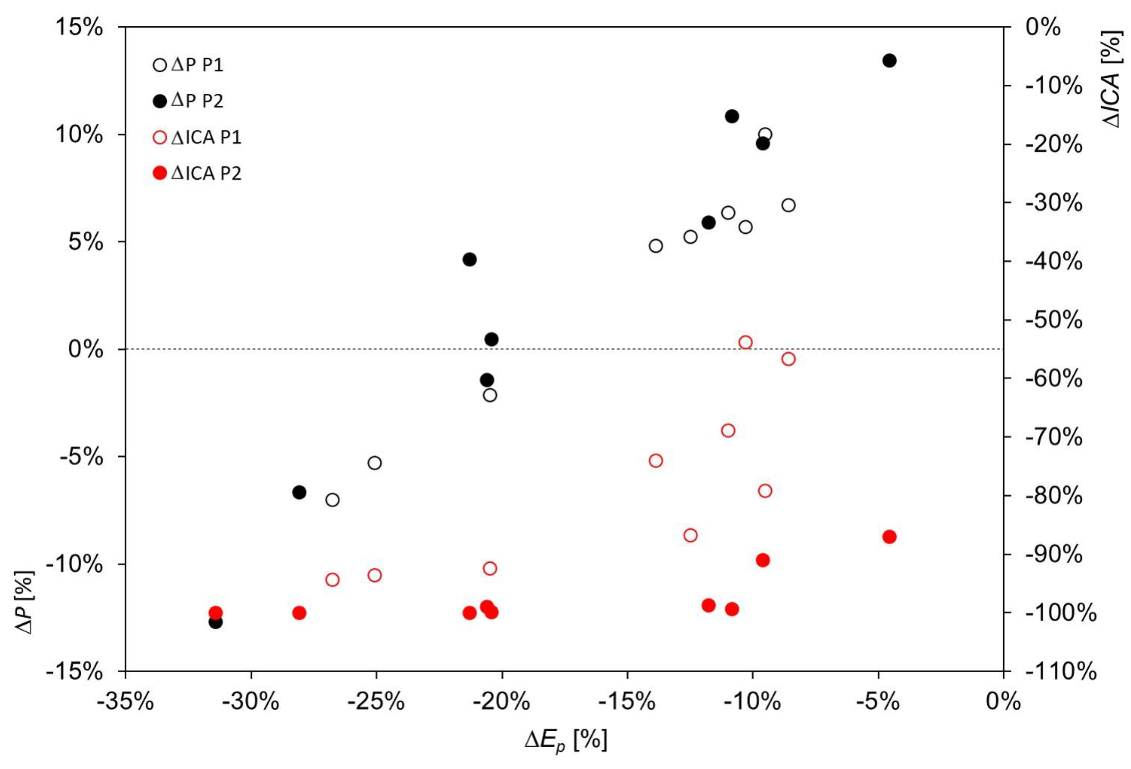
In Figure 13 we report a chart displaying ΔEp against ΔP (in Figure 7), and ΔICA (in Figure 10), in P1 (ICA in year 2051), and P2 (ICA in year 2092), in our nine scenarios (three GMCs, three RCPs). Therein, one clearly sees that energy production change is clearly positively linked to changes in precipitation. However, in those cases when precipitation is bigger than during CR period (ΔP > 0), still production may be smaller (ΔEp < 0). As an example in period P1, the smallest (in modulus) decrease of energy is ΔEp = −9%, given by RCP2.6 of ECHAM6 (see Figure 11) corresponds to an increase in total precipitation of ΔP = +6.7% (Figure 7), with a loss of ice cover ΔICA = −57% at that time (Figure 10). A similar situation occurs during P2, where even with an increase of rainfall ΔP = +13.4% under RCP2.6 of ECHAM6, energy production visibly decreases (ΔEp = −4.6%), as given by very large glacier’s down wasting, ΔICA = −87%. Looking at the scatter plot ΔICA in Figure 13 (red full dots), in period P2 at the end of century, ICA would be largely depleted (ΔICA = −100%). Looking at the corresponding scatter plot of ΔP for P2 (black full dots in Figure 13), one may roughly deduce that, in lack of glacier cover, with the present level of yearly precipitation (ΔP = 0), one would reach a lack of production nearby ΔEp = −20% or so. Accordingly, whenever precipitation would remain constant in the catchment until the end of the century, given large likelihood of glaciers’ large down wasting under any RCP scenario as demonstrated here, hydropower production would be decreasing. By still looking at the scatter plot of ΔP for P2 (black full dots in Figure 13), one may symmetrically hypothesize that roughly a ΔP = +20% would be necessary to achieve the present level of production.
Analysis of the seasonal reservoir’s level after Poly-Power management indicates on average (2005–2017) oscillation of the reservoir from a least volume in May (about 20 Mm3) after winter freeze, to a largest volume in September (about 25 Mm3) after summer thaw, despite maximum energy production during summer that is compensated by higher discharge values in that period.
Analysis of the yearly (2005–2017) reservoirs’ water balance (input volume minus output/hydropower volume, ΔV = Vin − Vout) indicates (not shown for shortness) extreme values of ΔV = −16.9 Mm3 to ΔV = +14.0 Mm3, corresponding respectively to −57%, and +47% of mean yearly flow E[Vin] = 29.7 Mm3, in the face of a reservoir’s volume of Vres = 44 Mm3.
Accordingly, the Sabbione reservoir can buffer, relatively well, variable flows from the catchment within the year, and even interannual variability therein, to provide optimal management for hydropower production.
However, visibly from our simulation, on the long run permanent lack of water as from our scenarios results into decreased production in spite of large buffer for regulation.
In turn, such lack of water clearly derives from decreased glacier extent over the century, and subsequent lack of cryospheric water.
In scenarios when large increase of precipitation would occur (here, up to +14% or so), increased availability of atmospheric water (rainfall, plus snow, melting at thaw), and proper regulation as here may partly make up for decreased ice melt. Conversely decreasing precipitation over the century would further affect hydropower production.
6.4. Limitations and Outlooks
Our study aimed at assessing the present, and future hydrological dynamics of the high altitude, poorly gauged (i.e., no stream flows, pool level, hydropower discharges available) Sabbione reservoir, paradigmatic of high altitude storage hydropower plants in the Alps. No information was available about catchment outflows given that (i) the catchment is closed by the lake and no measurable stream is present, and (ii) no (inverse) flow routing of the dam was possible to back-estimate input flows (e.g., [25]).
We were able to exploit topographic data, weather data recorded nearby (temperature, precipitation, snowfall), and ice ablation estimates of few seasons, to set up the Poly-Hydro model, capable of mimicking complex dynamics in high altitude cryospheric environment, and to subsequently validate it using ice cover estimates from remote sensing data, showing acceptable performance.
Cryospheric dynamic is here a very important driver of seasonal flows. Data from field campaigns and local stations, even if only for short periods, can be crucial to properly quantify ice/snow melt, and subsequently model hydrological fluxes (see for a discussion on this topic, e.g., [7,58]), so here we could originally exploit relevant information about snow, and especially ice contribution in this catchment, unmeasured hitherto that we know of.
We also neglected here flow routing, applied elsewhere (e.g., [8]), because no flow timing is available. Given that catchment flows are collected by the lake, and the considerable volume of the latter (Vres = 44 M m3), pool level is not largely affected by daily discharge (the maximum discharge estimated by the model during 2000–2017 may rise pool level by no more than 30 cm), so slight inaccuracy in daily discharge would not affect largely our operation.
Using Poly-Power model to calculate hydropower production under reservoir’s management, we reproduced acceptably well at least the sole available estimate of expected average production, so we are confident that our approach provides results that are representative of the glaciers/catchment/reservoir interaction.
The model of energy price we used takes in consideration only the effects of temperature rising, while it does not consider for example the impact of renewable energy sources that are expanding on the market and are usually not adjustable with demand but depends on weather conditions, which therefore can have an impact on energy price (e.g., [59]), and consequently on hydropower production optimization.
Our results regarding power production, albeit possibly inaccurate for the reasons previously exposed, may still be interesting for relative variations of hydropower potential under climate change scenarios, especially for the fact that use of Poly-Power allows to bypass the simplified, often unrealistic, assumption of run-of-river hydropower schemes, which likely provides less accurate assessment of hydropower production (and potential) in regulated systems.
While all GCMs and RCPs consistently project increased temperature over the century (Figure 7), precipitation projections are much more variable (Figure 7), with variation of ±15% or so.
Such issue is widely known to affect projection of future precipitation, in the Alps (e.g., [8,54,60]), and mountains worldwide [28,35,42], thus affecting projected hydrological behavior therein. Accordingly, one needs to explore an as large as possible array of conditions, as given by more GCMs/RCPs, to evaluate potential effects of different precipitation regimes.
Concerning meaning of RCPs, in principle all RCPs may be taken as equally likely to happen until the end of the century, so they represent equally plausible evolutions of climate, and of hydropower system in cascade. Among others however, recent findings [61] posed recent climate evolution somewhat more close to RCP8.5. Our results under that scenario point towards large loss of hydropower potential.
Future work may be therefore devoted to (i) more refined assessment of ice ablation, dynamics (velocity), and possibly thickness (e.g., via GPR, see [7]), (ii) recovery, whenever possible of pool level/hydropower flows for inverse flow routing, and production assessment, (iii) exploiting more climate scenarios/models, to explore large variability of weather projections, and a wider array of possible future evolutions (and possibly worst case scenarios), (iv) exploring potential adaptation strategies for hydropower management in a changing climate and mountain cryosphere.
7. Conclusions
The study presented here demonstrates the tight connection between cryospheric dynamics, hydrology, and hydropower production under present and perspective climate change in the high altitude Sabbione plant, paradigmatic of the hydropower system in Italian, and European Alps.
Given the complexity of cryospheric hydrology, local, data based, accurate modelling is necessary to quantify the nexus between climate, water fluxes, and production, and we demonstrated here use of Poly-Hydro model, well suited in this respect.
In addition, we used Poly-Power model, to assess optimal reservoir’s operation under present and future conditions, also considering explicitly the variability of energy prices against climate, and economic growth, often neglected in recent studies.
We demonstrated that hydropower potential until the end of century would decrease (−5% to −31%), this wide range depending upon (i) magnitude and of highly likely down wasting of glacier’s body, decreasing seasonal ice melt, and (ii) magnitude and direction of precipitation change, with potential of either positive or negative impact.
Our results indicate that research upon future water resources, and hydropower in high altitude with relevant cryospheric components as the Sabbione here is worthwhile, to substantiate assessment of hydropower potential in the years to come, where unless for exceptional hot years ice melt will be lower, and propose adaptation therein.
The water from Sabbione plant is collected by Morasco lake, which is artificially regulated itself and exploited for power production. As a further development it would be interesting to study the impact of climate change upon the two plants’ systems considered as a whole or exploring the possibility to install a pumped-storage system, i.e., using surplus energy from the electric system during periods of low demand to refill the reservoir as an adaptation strategy to climate change.
Other, more complex plants may have similarly decreasing potential in the future, but operation over a larger network may make up for modified hydrological cycle. Either way, knowledge of the expected water resources under future climate variations is necessary to design and test adaptation, maybe under a worst case scenario approach.
Under such perspective, (complex) re-operation of reservoirs will be increasingly important, and run-of-river schemes, as used at times now to evaluate hydropower potential will be less and less effective. Our study here provides therefore a tool to build knowledge of future expected hydrology, demand/price, and operation strategies in high altitude systems, and an application of an exemplary case study. Our tool, exportable to other similar catchments/reservoirs, may be of use for scientists, policy makers, hydropower companies, and in general for investigation of energy strategies for the future.
Author Contributions
Conceptualization, A.B., and D.B.; methodology, D.B.; software, G.M.B., L.S.; validation, L.S.; formal analysis, L.S.; investigation, L.S.; resources, D.B.; data curation, L.S., and G.M.B.; writing—original draft preparation, L.S.; writing—review and editing, D.B.; visualization, D.B.; supervision, A.B.; project administration, D.B.; funding acquisition, D.B.
Funding
This research received no external funding.
Acknowledgments
A. Tamburini of IMAGEO, and D. Catberro of SMI are kindly acknowledged for sharing information of Sabbione glacier’s GPR profiling. L. Mercalli, and P. Valisa of CGI are kindly acknowledged for sharing ice ablation data. R. Azzoni of University Milano is kindly acknowledged for help in photo interpretation for glacier’s area assessment. The present work reports results obtained in fulfilment of the lead author’s MS Thesis “La diga del ghiacciaio: cambiamenti climatici e produzione all’impianto del Sabbione”. The Thesis was awarded with the “MS Thesis Award of the Italian Glaciological Committee” for the year 2019. The authors kindly acknowledge support to the presented research from Politecnico di Milano under the Project: Climate-Lab, an Interdepartmental Laboratory on Global Climate Change at Polimi.
Conflicts of Interest
The authors declare no conflict of interest.
References
- Kaygusuz, K. Hydropower and the world’s energy future. Energy Sources 2004, 26, 215–224. [Google Scholar] [CrossRef]
- Ravazzani, G.; Dalla Valle, F.; Gaudard, L.; Mendlik, T.; Gobiet, A.; Mancini, M. Assessing climate impacts on hydropower production: The case of the Toce River Basin. Climate 2016, 4, 16. [Google Scholar] [CrossRef]
- Giuliani, M.; Anghileri, D.; Castelletti, A.; Vu, P.N.; Soncini-Sessa, R. Large storage operations under climate change: Expanding uncertainties and evolving tradeoffs. Environ. Res. Lett. 2016, 11, 035009. [Google Scholar] [CrossRef]
- Akbari-Alashti, H.; Soncini, A.; Dinpashoh, Y.; Fakheri-Fard, A.; Talatahari, S.; Bocchiola, D. Operation of two major reservoirs of Iran under IPCC scenarios during the XXI century. Hydrol. Process. 2018, 32, 3254–3271. [Google Scholar] [CrossRef]
- Gaudard, L.; Romerio, F. The future of hydropower in Europe: Interconnecting climate, markets and policies. Environ. Sci. Policy 2014, 37, 172–181. [Google Scholar] [CrossRef]
- Viganò, G.; Confortola, G.; Fornaroli, R.; Cabrini, R.; Canobbio, S.; Mezzanotte, V.; Bocchiola, D. Effects of future climate change on a river habitat in an Italian alpine catchment. J. Hydrol. Eng. 2015, 21, 04015063. [Google Scholar] [CrossRef]
- Soncini, A.; Bocchiola, D.; Azzoni, R.S.; Diolaiuti, G. A methodology for monitoring and modeling of high altitude Alpine catchments. Prog. Phys. Geogr. 2017, 41, 393–420. [Google Scholar] [CrossRef]
- Aili, T.; Soncini, A.; Bianchi, A.; Diolaiuti, G.; D’Agata, C.; Bocchiola, D. Assessing water resources under climate change in high-altitude catchments: A methodology and an application in the Italian Alps. Theor. Appl. Climatol. 2018, 135, 1–22. [Google Scholar] [CrossRef]
- D’Agata, C.; Bocchiola, D.; Soncini, A.; Maragno, D.; Smiraglia, C.; Diolaiuti, G.A. Recent area and volume loss of Alpine glaciers in the Adda River of Italy and their contribution to hydropower production. Cold Reg. Sci. Technol. 2018, 148, 172–184. [Google Scholar] [CrossRef]
- Maran, S.; Volonterio, M.; Gaudard, L. Climate change impacts on hydropower in an alpine catchment. Environ. Sci. Policy 2014, 43, 15–25. [Google Scholar] [CrossRef]
- Barry, R.G. The status of research on glaciers and global glacier recession: A review. Prog. Phys. Geogr. 2006, 30, 285–306. [Google Scholar] [CrossRef]
- Mann, M.E. Little ice age. In Encyclopedia of Global Environmental Change; Wiley: Chichester, UK, 2002; Volume 1, pp. 504–509. Available online: https://citeseerx.ist.psu.edu/viewdoc/download?doi=10.1.1.408.1689&rep=rep1&type=pdf (accessed on 31 July 2019).
- Oerlemans, J. Quantifying global warming from the retreat of glaciers. Science 1994, 264, 243–245. [Google Scholar] [CrossRef] [PubMed]
- Dyurgerov, M.B.; Meier, M.F. Twentieth century climate change: Evidence from small glaciers. Proc. Natl. Acad. Sci. USA 2000, 97, 1406–1411. [Google Scholar] [CrossRef] [PubMed] [Green Version]
- Maragno, D.; Diolaiuti, G.; D’agata, C.; Mihalcea, C.; Bocchiola, D.; Bianchi Janetti, E.; Smiraglia, C. New evidence from Italy (Adamello Group, Lombardy) for analysing the ongoing decline of Alpine glaciers. Geogr. Fis. Din. Quat. 2009, 32, 31–39. [Google Scholar]
- Diolaiuti, G.; Bocchiola, D.; D’agata, C.; Smiraglia, C. Evidence of climate change impact upon glaciers’ recession within the Italian Alps. Theor. Appl. Climatol. 2012, 109, 429–445. [Google Scholar] [CrossRef]
- Diolaiuti, G.A.; Bocchiola, D.; Vagliasindi, M.; D’agata, C.; Smiraglia, C. The 1975–2005 glacier changes in Aosta Valley (Italy) and the relations with climate evolution. Prog. Phys. Geogr. 2012, 36, 764–785. [Google Scholar] [CrossRef]
- IPCC. Summary for Policymakers. In Global Warming of 1.5 °C. An IPCC Special Report on the Impacts of Global Warming of 1.5 °C above Pre-Industrial Levels and Related Global Greenhouse Gas Emission Pathways, in the Context of Strengthening the Global Response to the Threat of Climate Change, Sustainable Development, and Efforts to Eradicate Poverty; Masson-Delmotte, V., Zhai, P., Pörtner, H.O., Roberts, D., Skea, J., Shukla, P.R., Pirani, A., Moufouma-Okia, W., Péan, C., Pidcock, R., et al., Eds.; World Meteorological Organization: Geneva, Switzerland, 2018; Volume 32, Available online: https://wg1.ipcc.ch/SR/documents/SR1.5_LAM3_Room_Assignment.pdf (accessed on 31 July 2019).
- Brunetti, M.; Lentini, G.; Maugeri, M.; Nanni, T.; Auer, I.; Boehm, R.; Schoener, W. Climate variability and change in the Greater Alpine Region over the last two centuries based on multi-variable analysis. Int. J. Climatol. 2009, 29, 2197–2225. [Google Scholar] [CrossRef]
- Zemp, M.; Paul, F.; Hoelze, M.; Haeberli, W. Glacier fluctuations in the European Alps, 1850–2000. In Darkening Peaks: Glacier Retreat, Science, and Society; Orlove, B., Wiegandt, E., Luckman, B.H., Eds.; University of California Press: Berkeley, CA, USA, 2008; pp. 152–167. ISBN 9780520235056. [Google Scholar]
- Smiraglia, C.; Diolaiuti, G.A. Il Nuovo Catasto dei Ghiacciai Italiani. [The New Italian Glacier Inventory]; EVK2CNR, Ed.; EVK2CNR: Bergamo, Italy, 2015; p. 400. ISBN 9788894090802. [Google Scholar]
- Smiraglia, C.; Diolaiuti, G.; Pelfini, M.; Belò, M.; Citterio, M.; Carnielli, T.; D’Agata, C. Glacier changes and their impacts on mountain tourism. In Darkening Peaks: Glacier Retreat, Science, and Society; Orlove, B., Wiegandt, E., Luckman, B.H., Eds.; University of California Press: Berkeley, CA, USA, 2008; pp. 206–215. ISBN 9780520235056. [Google Scholar]
- Meier, M.F. Contribution of small glaciers to global sea level. Science 1984, 226, 1418–1421. [Google Scholar] [CrossRef]
- Minora, U.; Senese, A.; Bocchiola, D.; Soncini, A.; D’agata, C.; Ambrosini, R.; Diolaiuti, G. A simple model to evaluate ice melt over the ablation area of glaciers in the Central Karakoram National Park, Pakistan. Ann. Glaciol. 2015, 56, 202–216. [Google Scholar] [CrossRef] [Green Version]
- Bocchiola, D.; Mihalcea, C.; Diolaiuti, G.; Mosconi, B.; Smiraglia, C.; Rosso, R. Flow prediction in high altitude ungauged catchments: A case study in the Italian Alps (Pantano Basin, Adamello Group). Adv. Water Resour. 2010, 33, 1224–1234. [Google Scholar] [CrossRef]
- Bocchiola, D. Long term (1921–2011) changes of alpine catchments regime in northern Italy. Adv. Water Resour. 2014, 70, 51–64. [Google Scholar] [CrossRef]
- Bombelli, G.M.; Soncini, A.; Bianchi, A.; Bocchiola, D. Potentially modified hydropower production under climate change in the Italian Alps. Hydrol. Process. 2019, 1–18. [Google Scholar] [CrossRef]
- Bocchiola, D.; Soncini, A.; Senese, A.; Diolaiuti, G. Modelling hydrological components of the Rio Maipo of Chile, and their prospective evolution under climate change. Climate 2018, 6, 57. [Google Scholar] [CrossRef]
- Groppelli, B.; Soncini, A.; Bocchiola, D.; Rosso, R. Evaluation of future hydrological cycle under climate change scenarios in a mesoscale alpine watershed of Italy. Nat. Hazards Earth Sys. Sci. 2011, 11, 1769–1785. [Google Scholar] [CrossRef]
- Mazza, A.; Mercalli, L. Il Ghiacciaio Meridionale dell’Hohsand (Alta Val Formazza): Un secolo di evoluzione climatica ei rapporti con la produzione idroelettrica. Oscellana 1992, 22, 30–44. [Google Scholar]
- Paro, L. Permafrost e forme periglaciali alle falde del corno di Ban. In L’ambiente Glaciale e Periglaciale dei Sabbioni (Hohsand). Formazza; Arpa Piemonte: Torino, Italy, 2012; 56p, Published in fulfilment of the Program: Interreg di cooperazione transfrontaliera Italia-Svizzera 2007–2013. In Italian; Available online: http://www.arpa.piemonte.it/pubblicazioni-2/pubblicazioni-anno-2012/sabbioni/at_download/file (accessed on 10 August 2019).
- Belotti, P.; Biagi, L.; Brovelli, M.A.; Campi, A.; Campus, S.; Cannata, M.; Credali, M.; Manzino, A.M.; Sansò, F.; Siletto, G.B. Introduzione al progetto HELI-DEM [An introduction to HELI-DEM project]. Bollettino della Società Italiana di Fotogrammetria e Topografia 2013, 13, 11–22. Available online: http://www.fondazionepolitecnico.it/uploads/test/SIFET_Il%20Progetto%20HELI-DEM.pdf (accessed on 31 July 2019).
- Bocchiola, D.; Rosso, R. The distribution of daily Snow Water Equivalent in the Central Italian Alps. Adv. Water Resour. 2007, 30, 135–147. [Google Scholar] [CrossRef]
- Valt, M.; Chiambretti, I.; Dellavedova, P. Fresh snow density on the Italian Alps. In Geophysical Research Abstracts; Copernicus: Göttingen, Germany, 2014; Volume 16, Available online: https://meetingorganizer.copernicus.org/EGU2014/EGU2014-9715.pdf (accessed on 31 July 2019).
- Soncini, A.; Bocchiola, D.; Confortola, G.; Minora, U.; Vuillermoz, E.; Salerno, F.; Diolaiuti, G. Future hydrological regimes and glacier cover in the Everest region: The case study of the upper Dudh Koshi basin. Sci. Total Environ. 2016, 565, 1084–1101. [Google Scholar] [CrossRef] [Green Version]
- Baldasso, V.; Soncini, A.; Azzoni, R.S.; Diolaiuti, G.; Bocchiola, D. Recent evolution of glaciers in Western Asia in response to global warming: The case study of mount Ararat, Turkey, Theoret. Appl. Climatol. 2018, 1–15. [Google Scholar] [CrossRef]
- Ente Nazionale Energia Elettrica ENEL, 2014. Morasco. Centrale Idroelettrica. Available online: https://web.archive.org/web/20140706072532/http://www.enel.it:80/it-IT/impianti/mappa/dettaglio/morasco-formazza/p/090027d98192f97b (accessed on 31 July 2019).
- IPCC. Summary for Policymakers. In Climate Change 2013: The Physical Science Basis. Contribution of Working Group I to the Fifth Assessment Report of the Intergovernmental Panel on Climate Change; Stocker, T.F., Qin, D., Plattner, G.-K., Tignor, M., Allen, S.K., Boschung, J., Nauels, A., Xia, Y., Bex, V., Midgley, P.M., Eds.; Cambridge University Press: Cambridge, UK; New York, NY, USA, 2013; Available online: http://www.climatechange2013.org/images/report/WG1AR5_Frontmatter_FINAL.pdf (accessed on 31 July 2019).
- Stevens, B.; Giorgetta, M.; Esch, M.; Mauritsen, T.; Crueger, T.; Rast, S.; Brokopf, R. Atmospheric component of the MPI-M earth system model: ECHAM6. J. Adv. Model. Earth Syst. 2013, 5, 146–172. [Google Scholar] [CrossRef]
- Hazeleger, W.; Severijns, C.; Semmler, T.; Ştefănescu, S.; Yang, S.; Wang, X.; Bougeault, P. EC-Earth: A seamless earth-system prediction approach in action. Bull. Am. Meteorol. Soc. 2010, 91, 1357–1364. [Google Scholar] [CrossRef]
- Groppelli, B.; Bocchiola, D.; Rosso, R. Spatial downscaling of precipitation from GCMs for climate change projections using random cascades: A case study in Italy. Water Resour. Res. 2011, 47, W03519. [Google Scholar] [CrossRef]
- Soncini, A.; Bocchiola, D.; Confortola, G.; Bianchi, A.; Rosso, R.; Mayer, C.; Lambrecht, A.; Palazzi, E.; Smiraglia, C.; Diolaiuti, G.A. Future hydrological regimes in the upper Indus basin: A case study from a high-altitude glacierized catchment. J. Hydrometeorol. 2015, 16, 306–326. [Google Scholar] [CrossRef]
- Haeberli, W.; Hölzle, M. Application of inventory data for estimating characteristics of and regional climate-change effects on mountain glaciers: A pilot study with the European Alps. Ann. Glaciol. 1995, 21, 206–212. [Google Scholar] [CrossRef]
- Oerlemans, J. Glaciers and Climate Change; August Aimé Balkema Publishers: Brookfield, VT, USA, 2001; p. 148. [Google Scholar]
- Bocchiola, D.; Soncini, A. Water Resources Modeling and Prospective Evaluation in the Indus River Under Present and Prospective Climate Change. In Indus River Basin; Elsevier: Amsterdam, The Netherlands, 2019; pp. 17–56. [Google Scholar] [CrossRef]
- Hargreaves, G.H. The estimation of potential and crop evapotranspiration. Am. Soc. Agric. Eng. Trans. 1974, 17, 701–704. [Google Scholar] [CrossRef]
- Bombelli, G.M.; Soncini, A.; Bianchi, A.; Bocchiola, D. Influence of climate change scenarios on energy price: A case study in Italy. Submitt. Environ. Model. Assess. 2018. submitted. [Google Scholar]
- Apadula, F.; Bassini, A.; Elli, A.; Scapin, S. Relationships between meteorological variables and monthly electricity demand. Appl. Energy 2012, 98, 346–356. [Google Scholar] [CrossRef]
- Grossi, G.; Caronna, P.; Ranzi, R. Hydrologic vulnerability to climate change of the Mandrone glacier (Adamello-Presanella group, Italian Alps). Adv. Water Resour. 2013, 55, 190–203. [Google Scholar] [CrossRef] [Green Version]
- Garavaglia, R.; Marzorati, A.; Confortola, G.; Bocchiola, D.; Cola, G.; Manzata, E.; Senese, A.; Smiraglia, C.; Diolaiuti, G.A. Evoluzione del ghiacciaio dei Forni. Neve Valanghe 2014, 81, 60–67. [Google Scholar]
- Diolaiuti, G.A. The recent reduction of the Lombardy glaciers: Results of the post recent mass balances. Geogr. Fis. Din. Quat. 2001, 5, 65–75. [Google Scholar]
- Cannone, N.; Diolaiuti, G.; Guglielmin, M.; Smiraglia, C. Accelerating climate change impacts on alpine glacier forefield ecosystems in the European Alps. Ecol. Appl. 2008, 18, 637–648. [Google Scholar] [CrossRef]
- D’Agata, C.; Bocchiola, D.; Maragno, D.; Smiraglia, C.; Diolaiuti, G.A. Glacier shrinkage driven by climate change during half a century (1954–2007) in the Ortles-Cevedale group (Stelvio National Park, Lombardy, Italian Alps). Theor. Appl. Climatol. 2014, 116, 169–190. [Google Scholar] [CrossRef]
- Confortola, G.; Soncini, A.; Bocchiola, D. Climate change will affect hydrological regimes in the Alps: A case study in Italy. J. Alpine Res. 2013, 101, 3–19. [Google Scholar] [CrossRef]
- Bavay, M.; Grünewald, T.; Lehning, M. Response of snow cover and runoff to climate change in high Alpine catchments of Eastern Switzerland. Adv. Water Resour. 2013, 55, 4–16. [Google Scholar] [CrossRef]
- Gaudard, L.; Gabbi, J.; Bauder, A.; Romerio, F. Long-term uncertainty of hydropower revenue due to climate change and electricity prices. Water Resour. Manag. 2016, 30, 1325–1343. [Google Scholar] [CrossRef]
- Gaudard, L.; Gilli, M.; Romerio, F. Climate change impacts on hydropower management. Water Resour. Manag. 2013, 27, 5143–5156. [Google Scholar] [CrossRef]
- Konz, M.; Seibert, J. On the value of glacier mass balances for hydrological model calibration. J. Hydrol. 2010, 385, 238–246. [Google Scholar] [CrossRef] [Green Version]
- Mulder, M.; Scholtens, B. The impact of renewable energy on electricity prices in the Netherlands. Renew. Energy 2013, 57, 94–100. [Google Scholar] [CrossRef]
- Faggian, P.; Giorgi, F. An analysis of global model projections over Italy, with particular attention to the Italian Greater Alpine Region (GAR). Clim. Chang. 2009, 96, 239–258. [Google Scholar] [CrossRef]
- Fuss, S.; Canadell, J.G.; Peters, G.P.; Tavoni, M.; Andrew, R.M.; Ciais, P.; Le Quéré, C. Betting on negative emissions. Nat. Clim. Chang. 2014, 4, 850–853. [Google Scholar] [CrossRef]
Figure 1.
Case study area. Sabbione artificial lake, and glaciers’ outline (in year 2000). Closest automatic weather station (AWS) station (Formazza) reported, used for weather driven Poly-Hydro simulation. On the lower right the red triangles are temperature station used for downscaling and the blue circle contains the Sabbione basin.

Figure 2.
Sabbione glacier. Initial condition of ice covered area ICA, and estimated ice thickness, year 2000.
Figure 2.
Sabbione glacier. Initial condition of ice covered area ICA, and estimated ice thickness, year 2000.

Figure 3.
Sabbione glacier. Simulated and observed ice covered area ICA, and estimated ice thickness in years 2007 (a), 2012 (b), 2015 (c), 2017 (d).
Figure 3.
Sabbione glacier. Simulated and observed ice covered area ICA, and estimated ice thickness in years 2007 (a), 2012 (b), 2015 (c), 2017 (d).

Figure 4.
Sabbione catchment. Estimated mean monthly flows (2000–2017). Estimated flow contributions (ice melt, snow melt, rainfall, ground flow) reported.
Figure 4.
Sabbione catchment. Estimated mean monthly flows (2000–2017). Estimated flow contributions (ice melt, snow melt, rainfall, ground flow) reported.

Figure 5.
Sabbione reservoir. Estimated mean monthly energy production Ep. Control Run (2005–2017), and projected. Period P1 (2045–2059).
Figure 5.
Sabbione reservoir. Estimated mean monthly energy production Ep. Control Run (2005–2017), and projected. Period P1 (2045–2059).

Figure 6.
Sabbione reservoir. Estimated mean monthly energy production Ep. Control Run (2005–2017) and projected. Period P2 (2086–2100).
Figure 6.
Sabbione reservoir. Estimated mean monthly energy production Ep. Control Run (2005–2017) and projected. Period P2 (2086–2100).

Figure 7.
Variables change along the century against the Control Run period (2000–2017 for T, P, Q, 2005–2017 for E). Periods P1 (2045–2059), and P2 (2086–2100) AWS Formazza. (a) Temperature change (°C). (b) Precipitation change (%). (c) Discharge change (%). (d) Energy production change (%).
Figure 7.
Variables change along the century against the Control Run period (2000–2017 for T, P, Q, 2005–2017 for E). Periods P1 (2045–2059), and P2 (2086–2100) AWS Formazza. (a) Temperature change (°C). (b) Precipitation change (%). (c) Discharge change (%). (d) Energy production change (%).

Figure 8.
Sabbione catchment. Estimated mean monthly, and yearly mean discharge Q (m3 s-1). Control Run (2005–2017) and projected for period P1 (2045–2059).
Figure 8.
Sabbione catchment. Estimated mean monthly, and yearly mean discharge Q (m3 s-1). Control Run (2005–2017) and projected for period P1 (2045–2059).

Figure 9.
Sabbione catchment. Estimated mean monthly, and yearly mean discharge Q (m3 s−1). Control Run (2005–2017) and projected for period P2 (2086–2100).
Figure 9.
Sabbione catchment. Estimated mean monthly, and yearly mean discharge Q (m3 s−1). Control Run (2005–2017) and projected for period P2 (2086–2100).

Figure 10.
Sabbione glacier. Estimated ice covered area ICA (km2), and mean yearly contribution of ice melt flow discharge Qice (%) until 2100. Control Run (2005–2017) and subsequently projected. ICA left y axis. Qice right y axis, upside-down.
Figure 10.
Sabbione glacier. Estimated ice covered area ICA (km2), and mean yearly contribution of ice melt flow discharge Qice (%) until 2100. Control Run (2005–2017) and subsequently projected. ICA left y axis. Qice right y axis, upside-down.

Figure 11.
Sabbione reservoir. Projected mean monthly energy price relative to annual mean (€/MWh), against the CR scenario for period P1 (2045–2059).
Figure 11.
Sabbione reservoir. Projected mean monthly energy price relative to annual mean (€/MWh), against the CR scenario for period P1 (2045–2059).

Figure 12.
Sabbione reservoir. Projected mean monthly energy price relative to annual mean (€/MWh), against the CR scenario for period P2 (2086–2100).
Figure 12.
Sabbione reservoir. Projected mean monthly energy price relative to annual mean (€/MWh), against the CR scenario for period P2 (2086–2100).

Figure 13.
Sabbione reservoir. Energy production changes ΔEp, against precipitation changes ΔP and ice cover changes ΔICA, in P1 (ICA in year 2051), and P2 (ICA in year 2092).
Figure 13.
Sabbione reservoir. Energy production changes ΔEp, against precipitation changes ΔP and ice cover changes ΔICA, in P1 (ICA in year 2051), and P2 (ICA in year 2092).


Table 1.
Formazza Pian dei Camosci, AWS station. Monthly average values of temperature (mean, minimum, maximum), and precipitation (rainfall, snow water equivalent SWE) registered during 2000–2017.
Table 1.
Formazza Pian dei Camosci, AWS station. Monthly average values of temperature (mean, minimum, maximum), and precipitation (rainfall, snow water equivalent SWE) registered during 2000–2017.
| Temperature (°C) | Precipitation (mm) | ||||
|---|---|---|---|---|---|
| Month | Mean | Max | Min | Rainfall | SWE |
| Jan | −7.3 | −3.0 | −11.4 | 5 | 104 |
| Feb | −7.3 | −2.1 | −11.6 | 8 | 124 |
| Mar | −4.5 | 1.3 | −9.0 | 15 | 147 |
| Apr | −1.8 | 3.9 | −6.0 | 29 | 171 |
| May | 2.1 | 7.4 | −1.8 | 129 | 243 |
| Jun | 6.2 | 10.6 | 2.3 | 143 | 154 |
| Jul | 8.0 | 11.5 | 4.2 | 142 | 142 |
| Aug | 7.9 | 11.1 | 4.5 | 161 | 164 |
| Sep | 4.5 | 7.8 | 1.2 | 124 | 133 |
| Oct | 1.5 | 5.3 | −1.9 | 87 | 137 |
| Nov | −3.2 | 0.7 | −6.7 | 25 | 217 |
| Dec | −6.2 | −2.2 | −10.1 | 6 | 123 |
Table 2.
AWS stations used for temperature lapse rate assessment.
| AWS | Latitude (°) | Longitude (°) | Altitude (m asl) |
|---|---|---|---|
| Agnel lake | 45°28′5″ N | 7°8′23″ E | 2304 |
| Monviso | 44°39′37″ N | 7°05′19″ E | 3325 |
| Moro pass | 45°59′49″ N | 7°58′35″ E | 2820 |
| Gastaldi lodge | 45°17′53″ N | 7°08′36″ E | 2659 |
| Vaccarone lodge | 45°09′15″ N | 6°54′59″ E | 2745 |
| Sommeiller | 45°07′54″ N | 6°50′34″ E | 2981 |
| Col Agnel | 44°40′51″ N | 6°58′43″ E | 2685 |
| Sestriere Banchetta | 44°57′54″ N | 6°54′36″ E | 2480 |
| Bocchetta delle Pisse | 45°52′32″ N | 7°54′04″ E | 2410 |
| SLFARO | 46°02′ N | 7°26′ E | 3301 |
| SLFGLA | 47°00′ N | 9°00′ E | 2909 |
| SLFSIM | 46°28′ N | 8°58′ E | 2580 |
| SLFSI2 | 46°28′ N | 8°59′ E | 2450 |
| SLFVAL | 46°31′ N | 8°38′ E | 2448 |
| SLFANV | 46° 9′ N | 7°35′ E | 2896 |
| SLFAN2 | 46°11′ N | 7°32′ E | 2630 |
| SLFAR2 | 46°18′ N | 7°33′ E | 2850 |
| SLFBED | 46°31′ N | 8°38′ E | 2962 |
| SLFBEL | 46°23′ N | 8°10′ E | 2556 |
| SLFBER | 46°26′ N | 10°00′ E | 2959 |
| SLFBE2 | 46°26′ N | 10°00′ E | 2450 |
| SLFBE3 | 46°26′ N | 9°55′ E | 2620 |
| SLFBR2 | 46°33′ N | 9°53′ E | 2510 |
| EGH | 46°30′ N | 8°17′ E | 2893 |
| SLFELA | 46°33′ N | 9°53′ E | 3114 |
| SLFTUM | 46°47′ N | 8°59′ E | 3050 |
| GOR | 45°59′ N | 7°47′ E | 3129 |
| SLFCHA | 46°23′ N | 7°09′ E | 2540 |
| CMA | 46°50′ N | 9°10′ E | 2480 |
| Formazza | 46°25′60″ N | 8°21′30″ E | 2453 |
Table 3.
Images used for glacier’s model validation.
| Date | Type | Source |
|---|---|---|
| 4 October 1999 | Orthophoto | BLOM-CGR |
| 8 September 2007 | Orthophoto | AGEA |
| 26 July 2012 | Orthophoto | AGEA |
| Summer 2015 | Orthophoto | Cons. TEA |
| 14 October 2017 | Satellite | SENTINEL |
Table 4.
Glacio-hydrological model parameters, and goodness of fit statistics. Thermal melt factor and radiation melt factor are both reported for ice and snow. Bold values are calibrated against observed values.
Table 4.
Glacio-hydrological model parameters, and goodness of fit statistics. Thermal melt factor and radiation melt factor are both reported for ice and snow. Bold values are calibrated against observed values.
| Parameter | Unit | Description | Value | Method |
| αci,s | (-) | Albedo, clean ice, snow | 0.3, 0.7 | [7] |
| TMFci,s | (mm d−1 °C−1) | Thermal melt factor, clean ice, snow | 5.3, 3.4 | ice stakes, AWS |
| RMFci,s | (mm d−1 W−1 m2) | Radiation melt factor, clean ice, snow | 0, 4 × 10⁻³ | ice stakes, nivometer |
| Fv | (%) | Vegetation cover, average | 22 | Land cover |
| K | (mm d−1) | Saturated conductivity | 4 | [8] |
| k | (-) | Ground flow exponent | 1.5 | [8] |
| WMax | (mm) | Max soil storage, average | 52 | land cover |
| θw,θs | (-) | Water content, wilting, field capacity | 0.15, 0.35 | [29] |
| Ks | (m−3 y−1) | Ice flow basal sliding coeff. | 1.5 × 10⁻²¹ | [8] |
| Kd | (m−1 y−1) | Ice flow internal deformation coeff. | 1.2 × 10⁻²⁴ | [8] |
| Goodness of fit | ||||
| Variable | Unit | Description | Bias (%) | NSE(R2) (-) |
| Mci | (mm d−1) | Ice ablation | 0.0 | 0.63 |
| Ms | (mm d−1) | Snow ablation Formazza | 4.0 | 0.86 |
Table 5.
Validation of the modelled ice covered area from Poly-Hydro at five dates during 2000–2017.
Table 5.
Validation of the modelled ice covered area from Poly-Hydro at five dates during 2000–2017.
| Date | ICA Mod. (km2) | ICA Obs. (km2) | Diff. Mod.–Obs. (%) |
|---|---|---|---|
| 1 January 2000 | 4.2 | 4.2 | 0% (setup) |
| 8 September 2007 | 3.6 | 3.6 | 0% |
| 26 July 2012 | 3.3 | 3.4 | −4% |
| 10 September 2015 | 3.1 | 3.0 | +3% |
| 10 October 2017 | 2.9 | 2.7 | +8% |
| ΔICA (2000–2017) | −1.3 | −1.5 | −13% |
| ΔICA% (2000–2017) | −31 | −36 | +5% |
Table 6.
Correlation analysis of changes in energy production Ep against climatic and hydrologic drivers, yearly scale. Below diagonal, Pearson correlation coefficients. Significant (α = 5%) correlation coefficients are in bold. p-values are above the diagonal.
Table 6.
Correlation analysis of changes in energy production Ep against climatic and hydrologic drivers, yearly scale. Below diagonal, Pearson correlation coefficients. Significant (α = 5%) correlation coefficients are in bold. p-values are above the diagonal.
| Variable | ΔEp% | ΔT% | ΔP% | ΔQ% | ΔICA% |
|---|---|---|---|---|---|
| ΔEp% | - | 0.007 | <10−4 | <10−4 | 0.014 |
| ΔT% | −0.616 | - | 0.063 | 0.005 | 0.043 |
| ΔP% | 0.958 | −0.447 | - | <10−4 | 0.097 |
| ΔQ% | 0.999 | −0.626 | 0.960 | - | 0.015 |
| ΔICA% | 0.569 | −0.482 | 0.404 | 0.563 | - |
© 2019 by the authors. Licensee MDPI, Basel, Switzerland. This article is an open access article distributed under the terms and conditions of the Creative Commons Attribution (CC BY) license (http://creativecommons.org/licenses/by/4.0/).
Share and Cite
MDPI and ACS Style
Stucchi, L.; Bombelli, G.M.; Bianchi, A.; Bocchiola, D. Hydropower from the Alpine Cryosphere in the Era of Climate Change: The Case of the Sabbione Storage Plant in Italy. Water 2019, 11, 1599. https://doi.org/10.3390/w11081599
AMA Style
Stucchi L, Bombelli GM, Bianchi A, Bocchiola D. Hydropower from the Alpine Cryosphere in the Era of Climate Change: The Case of the Sabbione Storage Plant in Italy. Water. 2019; 11(8):1599. https://doi.org/10.3390/w11081599
Chicago/Turabian StyleStucchi, Leonardo, Giovanni Martino Bombelli, Alberto Bianchi, and Daniele Bocchiola. 2019. "Hydropower from the Alpine Cryosphere in the Era of Climate Change: The Case of the Sabbione Storage Plant in Italy" Water 11, no. 8: 1599. https://doi.org/10.3390/w11081599
Note that from the first issue of 2016, this journal uses article numbers instead of page numbers. See further details here.