Hydrological Responses to the Future Climate Change in a Data Scarce Region, Northwest China: Application of Machine Learning Models

Abstract

Forecasting the potential hydrological response to future climate change is an effective way of assessing the adverse effects of future climate change on water resources. Data-driven models based on machine learning algorithms have great application prospects for hydrological response forecasting as they require less developmental time, minimal input, and are relatively simple compared to dynamic or physical models, especially for data scarce regions. In this study, we employed an ensemble of eight General Circulation Models (GCMs) and two artificial intelligence-based methods (Support Vector Regression, SVR, and Extreme Learning Machine, ELM) to establish the historical streamflow response to climate change and to forecast the future response under Representative Concentration Pathway (RCP) scenarios 4.5 and 8.5 in a mountainous watershed in northwest China. We found that the artificial-intelligence-based SVR and ELM methods showed very good performances in the projection of future hydrological responses. The ensemble of GCM outputs derived very close historical hydrological hindcasts but had great uncertainty in future hydrological projections. Using the variables of GCM outputs as inputs to SVR can reduce intermediate downscaling links between variables and decrease the cumulative effect of bias in projecting future hydrological responses. Future precipitation in the study area will increase in the future under both scenarios, and this increasing trend is more significant under RCP 8.5 than under scenario 4.5. The results also indicate the streamflow change will be more sensitive to temperature (precipitation) under the RCP 8.5 (4.5) scenario. The findings and approach have important implications for hydrological response studies and the evaluation of impacts on localized regions similar to the mountainous watershed in this study.

1. Introduction

Global climate change is considered one of the major threats to human survival and development. The Fifth Assessment Report (5AR) of the Intergovernmental Panel on Climate Change (IPCC) demonstrates unequivocally that the global-scale climate will continue to warm until the end of the 21st century. The surface temperature warming is predicted to be 1.1 to 2.6 °C under Representative Concentration Pathway (RCP) scenario 4.5 and 2.6 to 4.8 °C under RCP scenario 8.5 globally, relative to 1986–2005 [1]. These changes will be expected to reinforce the hydrological cycle by changing the precipitation regime, altering the streamflow, increasing evapotranspiration [2], potentially having significant implications for freshwater resources [3,4], and consequently, threatening the sustainability of the natural environment as well as people’s well-being [5,6]. Projection of future climate impact on the behavior of hydrological processes is therefore becoming increasingly essential for assessing the availability of surface water resources and formulating future climate change adaptation strategies [3,7,8]. Regional scale studies covering the individual watershed are more helpful for understanding local hydrological processes compared to those on the continental or global scales. Scientific approaches for improving the preciseness of existing methods for water availability, especially at local scales, are pertinent tools in core decision-making.

Climate projections are usually integrated with a hydrological model to assess the potential effects of climate change on hydrological components [9,10]. The General Circulation Model (GCM) projections need to be downscaled before they are applied to force a hydrological model due to their coarse spatial resolution, failure to capture the significant characteristics of climatic variables in the sub-grids of GCMs [11], and inability to generate local climate details to directly gather information for water resources planning and investigations at a local drainage or basin level. Dynamic and statistical downscaling are two commonly used methods in the bias correction of GCM outputs [12]. Statistical downscaling methods aim to establish empirical relationships between the historical large-scale GCM outputs and the local climate characteristics, requiring less computational capacity and technical expertise than dynamic downscaling, and being easily adaptable to local predictive scales, especially if there is sufficient historical data. They can be used to generate probability distribution functions to establish statistical relationships between GCM outputs and local-scale climate features based on observations [13]. Consequently, statistical downscaling of GCM outputs has been widely applied in a number of hydrological studies (e.g., [7,14,15,16]).

However, due to the complexity of climate systems, and since GCMs are theoretical mathematical descriptions of the system, future climate projections by GCMs contain a high level of uncertainty. Hence, the results of hydrological responses to future climate change largely depend on the results of the downscaled variables. In other words, the uncertainty of the downscaled meteorological variables from the selection of downscaling methods and GCM outputs can enlarge the future hydrological forecasting uncertainties due to the cumulative effect of bias. It should be noted that the performance of the physically based hydrological model with downscaled historical GCMs variables as inputs is usually poor when simulating historical streamflow compared with observed historical meteorology [17,18,19]. The major reason for this is that physically based hydrological models involve certain input variables, so the downscaling procedure can induce predictive uncertainty. Especially in a data scarce region, the use of the physically based hydrological model is limited by the availability of underlying data (e.g., soil properties, vegetation distribution, topography), and hydro-meteorological data, which induce a large amount of uncertainty. Thus, the model cannot determine the hydrological processes with certainty. In addition, the different model algorithms and input data reliabilities increases the potential uncertainty in future hydrological change projection [20]. These uncertainties lead to poor performance, and consequently, hydrological responses are infeasible.

Artificial intelligence (AI) models using machine learning algorithms can accurately capture and represent the complex relationships between input and output [21]. Some recent studies focused on the projection of future hydrology variability using artificial-intelligence-based methods including the artificial neural network (ANN), support vector machine (SVM), and extreme learning machine (ELM). Chen et al. downscaled daily precipitation from large-scale weather variables using the SVM–based method. The model results were compared with the results of a statistical downscaling model, which showed that the SVM reproduced the most reasonable daily precipitation [13]. To capture the nonlinear variability between hydro–climate response variables and projectors, Sarhadi et al. proposed a new approach which was called “Supervised Principal Component Analysis (Supervised PCA)” for GCM outputs regression–based statistical downscaling [22], and then two machine learning models (Support Vector Regression and Relevance Vector Machine) were used to project the monthly precipitation [23]. Srinivas et al. presented a least-square support vector machine (LS–SVM)-based methodology for multi–site downscaling of daily temperature series [24]. Su et al. used ANN-based model to project precipitation and streamflow in the Songhuajiang River basin, China, in which multi-layer perceptron networks were applied to construct relationships between climate factors and hydrological variables [25]. These studies established the relationships between GCMs and hydrological components in a historical period and projected the future hydrological response under GCM emission scenarios [13,22,23,24,25]. ANN and SVM play key roles in machine learning and data analysis [26]. The SVM model presents an advancement over the conventional ANN model [27], whereas the ELM model offers an improvement in terms of its design and universal approximation capability, as it is a fast and efficient neuro-computational approach [28]. These methods are easy to operate, even for large basins, and have acceptable levels of accuracy, especially for data scarce regions. Since the inputs of these AI-based methods are flexible, the projection performance of the future hydrological responses using downscaled predictors or by directly selecting GCM output variables as inputs should be compared with observed hydrological components as predictands in the historical period.

Based on the above, the main aim of this paper is to integrate GCM outputs with AI-based models to directly estimate the potential hydrological response in a data scarce region. The sub-objects of this study are (1) to reduce the uncertainty of future hydrological simulation by selecting an ensemble of eight GCM outputs, (2) to compare the performance of the projections with two AI-based models (SVR and ELM) and two input datasets, (3) to compare the hydrological response in different RCP scenarios, and (4) to understand and detect the implications of future climate change on local-scale surface water availability in an alpine data scarce watershed in northwest China.

2. Materials and Methods

2.1. Study Area

The upper watershed of the Heihe River was selected as the study region (Figure 1). The Heihe River is located on the north slope of the Qilian Mountains, lying between 38° to 39° N and 99° to 101° E, and has a total surface area of 10,009 km². It is the transition zone between the prevailing high latitude westerlies and Asian summer monsoon, rendering this region complex and sensitive to climate change. The streamflow generated in the region is the major water resource (90%) for the entire Heihe River basin. The climate is characterized by cold and dry conditions in winter and warm and humid conditions in summer with large spatial and temporal heterogeneity. The multi-year average air temperature ranges from −5 to 4 °C. The air temperature increased by 0.37 °C/10yr in 1980–2010, which is faster than the rate over the last 60 years by 0.30 °C/10yr [29]. The multi-year average annual precipitation exceeds 400 mm, increasing by 15.5–16.4 mm for every 100 m rise in altitude. The precipitation increased more significantly (15.7 mm/10yr) in 1980–2010 than in the last 50 years (14.9 mm/10yr). The average annual runoff is 16.05 × 10⁸ m³ with significant inter-annual variation. Climate change has been the main cause of streamflow variation over the last 30 years [30]. In the last 50 years, climate change has contributed to an increase in the total streamflow by 14.08% [29].

2.2. Data Collection

2.2.1. Observed Data

In this study, the historical monthly precipitation and air temperature data from six national standard meteorological stations in and around the study area were collected from the China Meteorological Administration (CMA), with the data periods from 1961 to 2013 for four stations and 1995 to 2013 for the other two stations. The monthly streamflow data at the Yinluoxia Hydrological gauging station for 1961 to 2013 was obtained from the hydrological bureau of Gansu province to establish the historical climate–hydrological relationship and to investigate the suitable monthly lag time in precipitation and streamflow. The observed streamflow series was also used for calibration and validation of the historical hindcast streamflow results with the ensemble of GCM forcing data. The basic information of the observation stations is shown in

Table 1. Properties of the hydrometeorological stations in and around the upper watershed of Heihe River.

Station	Gauging Subject	Latitude/°	Longitude/°	Elevation/m	Time Span
Zhangye	Meteorology	38.9	100.4	1482.7	1961–2013
Sunan	Meteorology	38.8	99.6	2312	1995–2013
Minle	Meteorology	38.5	100.8	2271	1995–2013
Tuole	Meteorology	38.8	98.4	3367	1961–2013
Yeniugou	Meteorology	38.4	99.6	3320	1961–2013
Qilian	Meteorology	38.2	100.3	2787.4	1961–2013
Yingluoxia	Hydrology	38.8	100.18	1674	1961–2013

.

2.2.2. Coupled Model Intercomparison Project Phase-5 (CMIP5) Scenarios

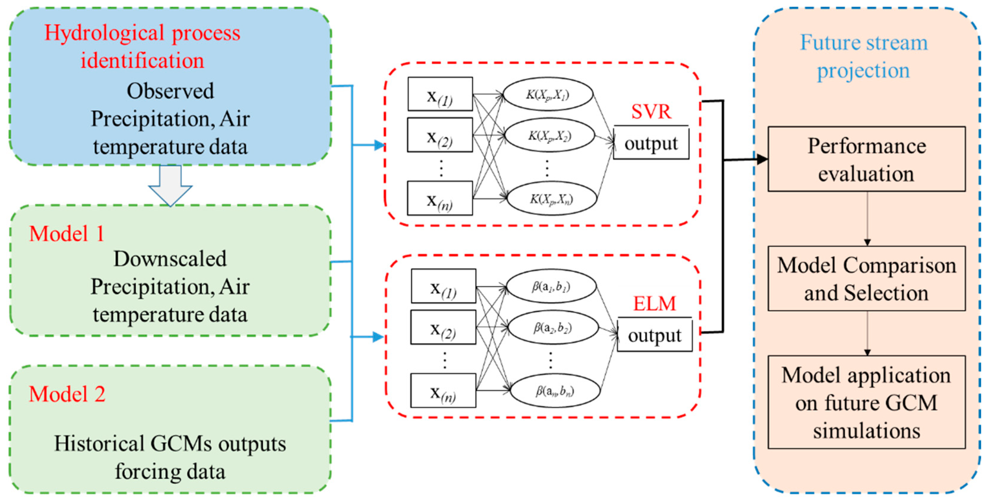
To yield an extensive evaluation and applicability of the downscaling techniques and to induce the uncertainty sourced from GCMs, a set of eight projections of the atmospheric climate variables generated from the newest version of CMIP5 were adopted in this study, namely ACCESS1.0, ACCESS1.3, BCC-CSM1.1(m), CNRM-CM5, HadGEM2-CC, HadGEM2-ES, MIROC5, and MRI-CGCM3. The future climate change simulations were thus employed for a period in the 21st century through different radiative forcing scenarios known as “Representative Concentration Pathways” (RCPs), which are designed to provide a consistent combination of future population growth and social and economic developments with the specified radiative forcing pathways [31]. The two radiative forcing scenarios considered in the present study are the RCP 4.5, which is a stabilization scenario where the radiative forcing is estimated to be about 4.5 W m⁻² by the end of 21st century, and the RCP 8.5, which is a high emission scenario with a radiative forcing of 8.5 W m⁻² before the year 2100.

The ACCESS1.0 and ACCESS1.3 models are two versions of the Australian Community Climate and Earth-System Simulator (ACCESS) which were jointly developed by the Commonwealth Scientific and Industrial Research Organization (CSIRO) and the Bureau of Meteorology (BOM) of Australia. The major components that make up the ACCESS climate models, including the principal differences between the ACCESS1.0 and ACCESS1.3 models, can be found in Collier and Uhe [32]. The BCC-CSM1.1(m) used in this study is version 1.1 of the Beijing Climate Center (BCC) Climate System Model (BCC-CSM1.1) and has a moderate atmospheric resolution. The atmospheric component, ocean component, land component, and sea component are fully coupled and interact with each other through fluxes in momentum, energy, water, and carbon at their interfaces. Detailed information about the BCC-CSM1.1 model can be found in [33,34]. CNRM-CM5, including the atmospheric model ARPEGE-Climat (v5.2), the ocean model NEMO (v3.2), the land surface scheme ISBA, and the sea ice model GELATO (v5) coupled through the OASIS (v3) system developed at the Centre Européen de Recherche et de Formation Avancée (CERFACS). The study presented in [35] described the framework of the CNRM-CM5 model and evaluated the model performance. HadGEM2-CC and HadGEM2-ES are two models of the HadGEM2 model family. The HadGEM2 family of model configurations includes atmosphere, ocean, and sea-ice components with and without vertical extension of the atmosphere model to include a well-resolved stratosphere and Earth System components including the terrestrial and oceanic carbon cycle (HadGEM2-CC) and tropospheric chemistry (HadGEM2-ES) [36]. The MIROC5 model is a new version of the atmosphere–ocean general circulation model which was cooperatively produced by the Japanese research community and was designed for the Intergovernmental Panel on Climate Change (IPCC) Fifth Assessment Report (AR5). The components and parameterization schemes included in MIROC5 were described in [37]. The MRI-CGCM3 was developed at the Meteorological Research Institute (MRI) and consists of the atmosphere-land model (MRI-AGCM3), the ocean and sea ice model (MRI.COM3), and the aerosol model (MASINGAR mk–2) [38].

The eight GCM models were used to perform experiments in the framework of CMIP5 [31]. The spatial resolution and data length are also shown in

Table 2. The Coupled Model Inter-comparison Project Phase-5 (CMIP5) model attributes selected in this study.

No.	Model	Modeling Centre	Spatial Resolution	Data Length
				Historical	RCP 4.5	RCP 8.5
1	ACCESS1.0	CSIRO-BOM (Australia)	1.875° × 1.25°	1948–2005	2006–2100	2006–2100
2	ACCESS1.3	CSIRO-BOM (Australia)	1.875° × 1.25°	1948–2005	2006–2100	2006–2100
3	BCC-CSM1.1(m)	BCC (China)	1.125° × 1.125°	1948–2005	2006–2100	2006–2100
4	CNRM-CM5	CNRM-CERFACS (France)	1.400° × 1.400°	1948–2005	2006–2100	2006–2100
5	HadGEM2-CC	MOHC (UK)	1.875° × 1.25°	1948–2005	2006–2100	2006–2100
6	HadGEM2-ES	MOHC (UK)	1.875° × 1.25°	1948–2005	2006–2100	2006–2100
7	MIROC5	CCSR (Japan)	1.400° × 1.400°	1948–2005	2006–2100	2006–2100
8	MRI-CGCM3	MRI (Japan)	1.125° × 1.125°	1948–2005	2006–2100	2006–2100

. According to the time series of observed data, we selected the data from 1961 to 2005 for historical experiment and the data from 2006 to 2100 for RCP scenarios 4.5 and 8.5 experiments.

2.3. Methodology

In data scarce regions, such as northwest China, the hydrological simulation accuracy of physically based distributed models is usually questionable due to the lack of regional parameter observations. Thus, in this study, we adopted the widely used machine learning methods (Extreme Learning Machine and Support Vector Regression) to establish lumped mathematical relationships between climatic predictors and streamflow at the monitoring station and to forecast the future streamflow in the upper watershed of Heihe River under the assumption of the validity of these relationships under a changing climate in the future.

2.3.1. Extreme Learning Machine

The extreme learning machine (ELM) is an efficient learning-algorithm-based tool that uses a single-hidden-layer feedforward neural networks (SLFN) architecture with numerous advantages including ease of use, quick learning speed, higher performance, and suitability for many nonlinear activation and kernel functions [39]. It is capable of determining all of the network parameters analytically, which prevents trivial human intervention. There are three layers in the ELM model, including the input layer, hidden layer, and output layer, and one of the significant factors is that the hidden layer does not need to be tuned. ELM randomly selects the input weights and then analytically determines the output weights of the SLFNs [40,41,42,43].

Given n training samples $\mathit{X}i={\left[x_{i1},x_{i2},\cdots ,x_{in}\right]}^T$, the output function for SLFNs with L hidden nodes can be expressed as

$$f_L\left(x\right)={\displaystyle \sum }_{i=1}^{i=L}{\beta }_i{h}_i\left(x\right)$$

(1)

where ${\beta }_i$ is the output weight of the $i^{th}$ hidden node, $h_i\left(x\right)$ is the hidden layer output mapping of ELM, representing the randomized hidden features of predictor $\mathit{X}i$, and $h_i\left(x\right)$ is the $i^{th}$ non-linear piecewise-continuous hidden layer activation function, given as

$${\mathit{h}}_{\mathit{i}}\left(x\right)=\mathit{G}\left({\mathit{a}}_{\mathit{i}},{\mathit{b}}_{\mathit{i}}\mathrm{X}\right)$$

(2)

where ${\mathit{a}}_{\mathit{i}}$ and ${\mathit{b}}_{\mathit{i}}$ are two hidden neuron parameters. The model’s approximation error is minimized when solving for weights connecting the hidden and output layer $\left(\beta \right)$ using a least-squares method, and its objective function is given as

$$\underset{\beta \in R^{L\times m}}{\min }{\Vert H\beta -T\Vert }^2$$

(3)

where $H$ is the hidden layer output matrix:

$$H=\left[\begin{array}{c}g\left(x_1\right)\\ ⋮\\ g\left(x_N\right)\end{array}\right]=\left[\begin{array}{ccc}{g}_1\left(a_1{x}_1+b_1\right)& \cdots & g_L\left(a_L{x}_1+b_L\right)\\ ⋮& \cdots & ⋮\\ g_1\left(a_N{x}_N+b_1\right)& \cdots & g_L\left(a_L{x}_N+b_L\right)\end{array}\right].$$

(4)

$T$ is the training target matrix:

$$T=\left[\begin{array}{c}{t}_1^T\\ ⋮\\ t_N^T\end{array}\right]=\left[\begin{array}{ccc}{t}_{11}& \cdots & t_{1m}\\ ⋮& \cdots & ⋮\\ t_{N1}& \cdots & t_{Nm}\end{array}\right].$$

(5)

2.3.2. Support Vector Regression

Support Vector Regression (SVR), an alternative form of the Support Vector Machine (SVM), is a novel machine learning technique that deals with the regression-based modeling process. For the case of regression approximations, suppose there is a given set of data points $G=\left\{\left(x_i,y_i\right)\right\}{n}_i$ ($x_i$ is the input vector; $y_i$ is the desired value; and $n$ is the total number of data points). To solve a nonlinear regression problem, the inputs are firstly nonlinearly mapped into a high-dimension feature space where they are correlated linearly with the output (target). The following linear estimation function can be employed to formalize the SVR model:

$$f\left(x\right)=\omega ·\varnothing \left(x\right)+b$$

(6)

where $\omega$ is weight vector, $b$ is a constant, and $\varnothing \left(x\right)$ denotes a mapping function in the feature space. The coefficients $\omega$ and $b$ can be estimated by minimizing

$$R_{reg}\left(f\right)=C\frac{1}{N}{\displaystyle \sum }_{i=1}^N{L}_{\epsilon }\left(f\left(x_i\right),y_i\right)+\frac{1}{2}{\Vert w\Vert }^2$$

(7)

$$L_{\epsilon }\left(f\left(x\right)-y\right)=\{\begin{array}{c}\left|f\left(x\right)-y\right|-\epsilon for\left|f\left(x\right)-y\right|\ge \epsilon \\ 0otherwise\end{array}$$

(8)

where both $C$ and $\epsilon$ are prescribed parameters. The first term $L_{\epsilon }\left(f\left(x_i\right),y_i\right)$ is called the ε-intensive loss function. This function indicates that errors below $\epsilon$ are not penalized. The term $C\frac{1}{N}{{\displaystyle \sum }}_{i=1}^N{L}_{\epsilon }\left(f\left(x_i\right),y_i\right)$ is the empirical error. The term $\frac{1}{2}{\Vert w\Vert }^2$ measures the smoothness of the function. $C$ evaluates the trade-off between the empirical risk and the smoothness of the model. The positive slack variables $\xi$ and ${\xi }^{*}$ represent the distance from the actual values to the corresponding boundary values of ε-tube. Equation (7) is transformed to the following constrained formation

$$\min \frac{1}{2}{\Vert w\Vert }^2+C{{\displaystyle \sum }}_{i=1}^N\left({\xi }_i+{\xi }_i^{*}\right)$$

(9)

$$\mathrm{subject}\mathrm{to}\{\begin{array}{c}{y}_i-\left(\langle w,x_i\rangle +b\right)\le \epsilon +{\xi }_i\\ \langle w,x_i\rangle +b-y_i\le \epsilon +{\xi }_i^{*}\\ {\xi }_i,{\xi }_i^{*}\ge 0\end{array}.$$

(10)

After taking the Lagrangian and optimal conditions, a nonlinear regression function is obtained using the following expression:

$$f\left(x\right)={{\displaystyle \sum }}_{i=1}^l\left({\alpha }_i-{\alpha }_i^{*}\right)k\left(x_i,x\right)+b$$

(11)

where ${\alpha }_i$ and ${\alpha }_i^{*}$ are the introduced Lagrange multipliers. With the utilization of the Karush–Kuhn–Tucker (KKT) conditions, only a limited number of coefficients will not be zero among ${\alpha }_i$ and ${\alpha }_i^{*}$. The related data points can be referred to as support vectors. $k\left(x_i,x\right)$ refers to kernel function, describing the inner product in the D-dimension feature space:

$$k\left(x,y\right)={{\displaystyle \sum }}_{i=1}^D{\varnothing }_j\left(x\right){\varnothing }_i\left(y\right).$$

(12)

Equation (12) shows that any symmetric kernel function k satisfying Mercer’s condition corresponds to a dot product in some feature space. In this paper, the radius basis function (RBF) is selected as the kernel function. The RBF is defined as follows:

$$k\left(x,y\right)=\exp \left(-\gamma {\Vert x-y\Vert }^2\right),\lambda >0.$$

(13)

It is important to note that when the RBF kernel is used in an SVR model, three parameters, including the penalty parameter C and the kernel function’s parameter $\mathsf{\gamma }$, are considered. The general performance of SVM models depends on the proper setting of these parameters, which are usually attained through a grid search process that minimizes the mean square error in the training dataset [13].

2.3.3. Model Development and Validation

The main purpose of this study was to accurately forecast the hydrological response to future climate change. Thus, we also applied ELM and SVR to establish the relationship between hydrological components and climate predictors in the historical period and forecast under future climate scenarios. A schematic diagram for future hydrological response projection was presented in Figure 2. Firstly, we employed the observed precipitation and temperature data as inputs to drive the machine learning models to evaluate the rainfall–runoff relationship in the study area. Considering that different inputs can directly affect the forecast results, we tried to compare the results of using downscaled climate data and direct GCMs outputs on historical hydrological hindcasting. Thus, two input datasets were built for each GCM. Model 1 included precipitation and air temperature data downscaled by ELM and SVR using GCM outputs, and Model 2 directly used historical GCM outputs. Each model used eight ensemble GCMs as input to derive the ELM and SVR with the observed monthly streamflow as the output target. Finally, after the comparison and selection of the higher performance inputs and modeling combination, we applied the future GCM outputs scenarios to project future hydrological responses. Thus, we divided the 45-year historical data set representing the current climate (1961–2005) into two sub-period datasets. The first 30 years of data (1961–1990) were used to develop and calibrate the regression model, while the remaining 15 years of data (1991–2005) were used to validate the model.

Four statistics, namely the correlation coefficient (R), the coefficient of the Nash–Sutcliffe efficiency (NSE), the root mean square error (RMSE), and the mean absolute relative error (MAE) were used to quantitatively assess the performance of the ELM and SVR results. R and NSE values close to 1 and RMSE and MAE values close to 0 indicate a more accurate model performance. Moreover, to investigate the variability of future hydrological projections, we employed the Sen Slope method and the M–K Test. The detailed information is shown in [44].

3. Results

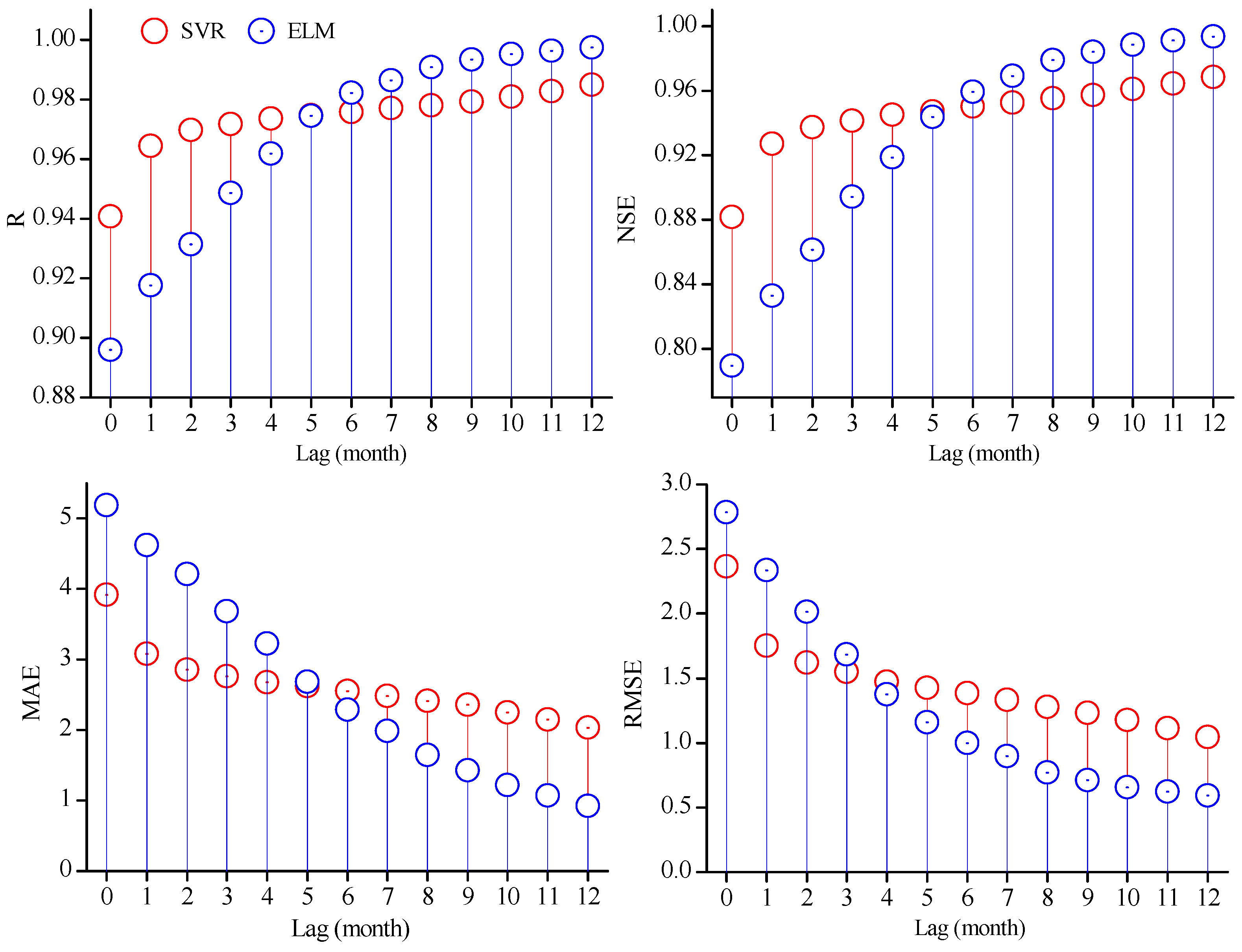
3.1. Climatic–Hydrological Relationship Identification

Before using the SVR and ELM to project future hydrological responses, the regional climate–hydrological relation should be first identified due to the streamflow always lags behind precipitation. Thus, we used the observed monthly precipitation and temperature as inputs to drive the SVR and ELM and considered the time lag of streamflow. Figure 3 shows the modeling performances of SVR and ELM derived from the observed monthly precipitation and temperature for different streamflow month lags. We can see that when the time lag was not considered, the modeling streamflow was worse than when the streamflow time lag was considered. When considering the steamflow time lag, the modeling results apparently improved. With the addition of the steamflow monthly lag, the modeling performance increased continuously, and this increasing situation was more significant for ELM than for SVR. When the streamflow time lag was close to 5 months, the two models had similar performances and these performances also satisfactorily represented the relation between observed monthly climatic predictors and the streamflow. In fact, the streamflow delay resulted mainly from precipitation infiltration, soil water movement, and groundwater return. The time lag we investigated was similar to that used in the distributed hydrological model for this area [30]. Thus, we selected 5 months as the streamflow monthly time lag to establish the historical climate–hydrology relationship.

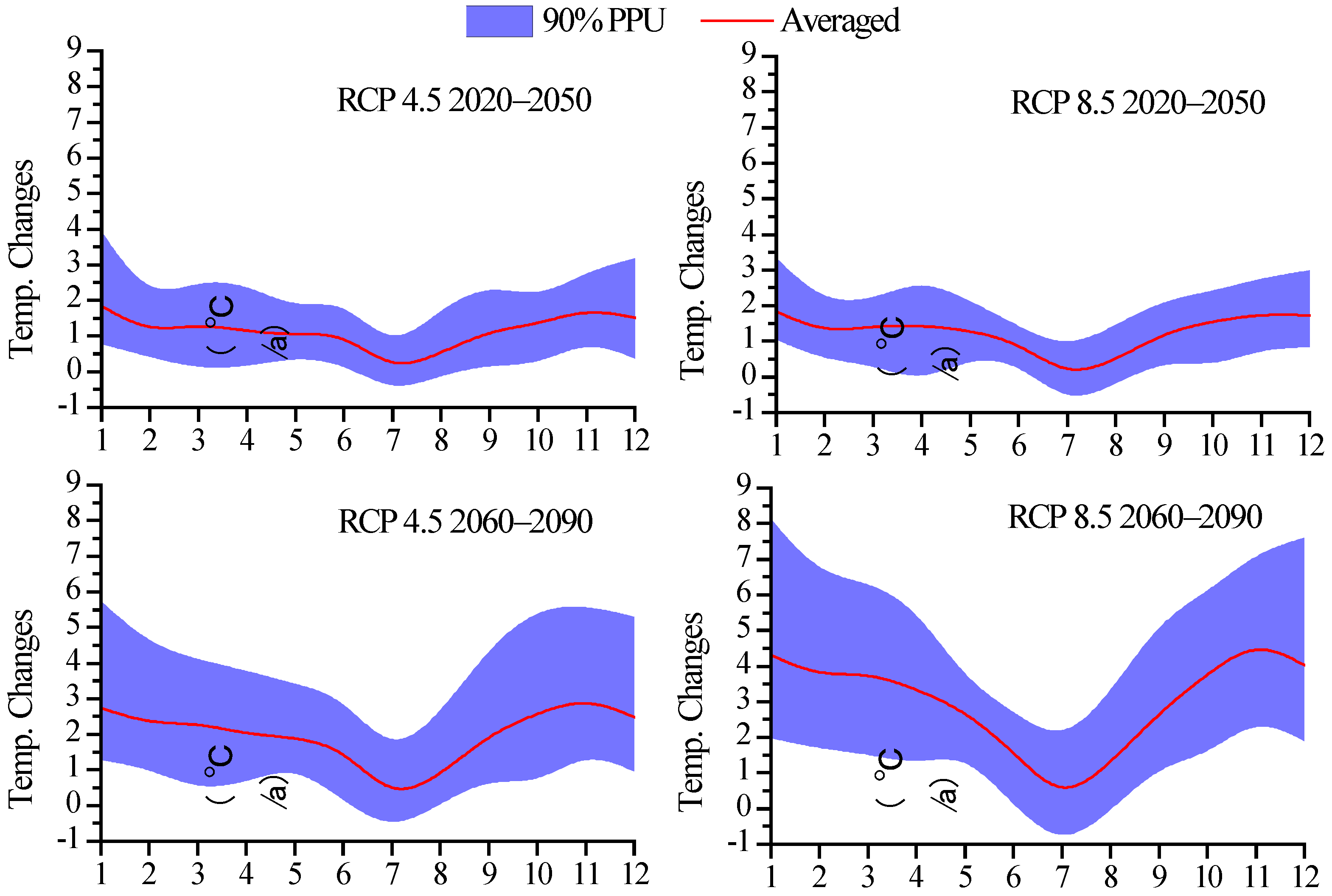
3.2. Future Temperature and Precipitation Forecasting

3.2.1. Future Temperature Forecasting

The projected annual time series of temperature and precipitation under RCP scenarios 4.5 and 8.5 (left panel) as well as the future changes (right panel) were determined using an ensemble of the average results derived from eight GCM outputs, as shown in Figure 4. We can see that the annual temperature continuously increases under both scenarios. For the near-term time projection (2020–2050), the average temperatures are similar for both scenarios. However, for the long-term projection (2060–2090), the average temperature for the RCP 8.5 scenario is larger than that for the RCP 4.5 scenario. With respect to the current climate (1961–2005), the temperature increases in the near term by a median of 1.1 °C and 1.3 °C for RCP scenarios 4.5 and 8.5, respectively, and it increases in the long term by a median of 1.7 °C and 2.9 °C for the RCP scenarios 4.5 and 8.5, respectively.

Figure 5 represents the future change tendency in the monthly temperature at different periods and climate scenarios, as simulated by Sen Slope methods. The change trends in temperature show great differences at the monthly scale. For both RCP scenarios, the temperature median trends are all positive for all months, with higher values in the long term under RCP scenario 8.5. The trends in the cold months are higher than those in the warm months for each period and RCP scenario. The shape of the inner-annual temperature change distribution is just like a “V”. This indicates that the temperature change in the cold season is more significant than that in the warm season. This corresponds to the historical temperature change studies by Yin et al. [29] and Yang et al. [30].

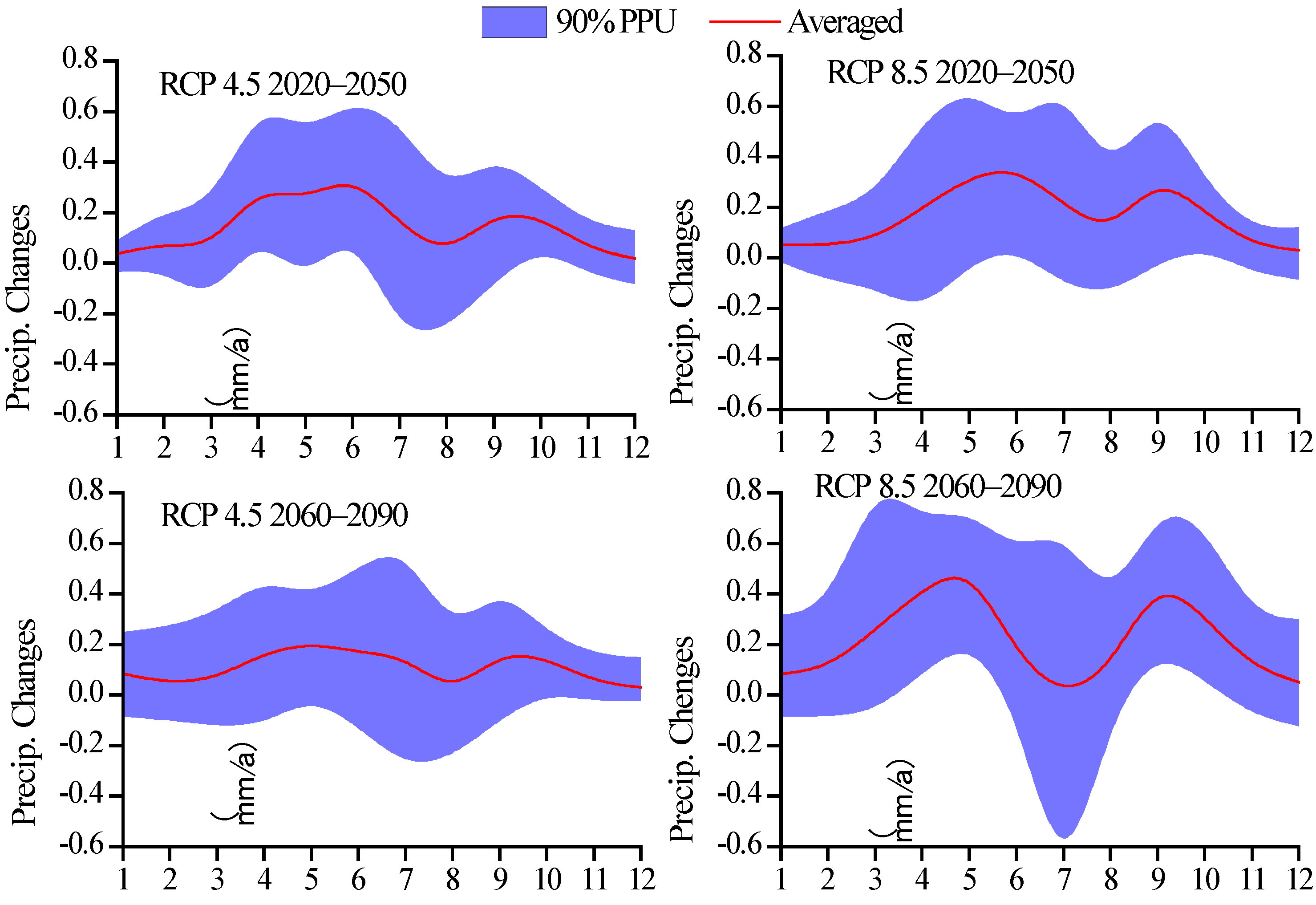
3.2.2. Future Precipitation Forecasting

The projected annual time series of precipitation and future change by the ensemble of average results derived from eight GCM outputs under RCP scenarios 4.5 and 8.5 are shown in Figure 4. We can see that from 2020 to 2100, the annual precipitation is predicted to exhibit increasing trends for both scenarios. Compared to the results under RCP scenario 4.5, the future precipitation under RCP scenario 8.5 shows more obvious uncertainty variation with less precipitation in the near term and higher precipitation in the long term. This uncertainty also increases as the time increases. To reduce the uncertainty of the single GCM, we applied the ensemble average value of the eight simulated results to represent the future projection in this study. There was an evident increasing trend in future precipitation under RCP scenario 8.5 comparing to under RCP scenario 4.5, especially near the end of the 21st century. It was found that the average precipitation under RCP 4.5 was 590 mm and 640 mm for the near- and long-term forecasts, respectively, and 605 mm and 720 mm under RCP scenario 8.5 for the near- and long-term forecasts, respectively.

The period from 1961 to 2005 was considered the baseline from which future changes in precipitation were evaluated. In Figure 4 (right panel), we illustrate the projected variation in annual precipitation (%) for the near- and long-term forecasts. Evidently, the precipitation is predicted to increase in the future under both scenarios. We can see that the precipitation increases by 15% in the near term and by 18% in the long term under RCP scenario 4.5. Notably, the increase in precipitation under RCP scenario 8.5 is more distinct than that under RCP scenario 4.5, with 21% and 33% for the near- and long-term forecasts, respectively. Figure 6 shows the median of the estimated slope trends of monthly precipitation generated from the projection pf precipitation in two periods and RCP scenarios. The monthly median precipitation trends all show increases, while in April, May, June, September, and October, the increasing trends are more obvious than those in the other months. This means the precipitation will tend to become more even in the future, and the drought in spring will be relieved.

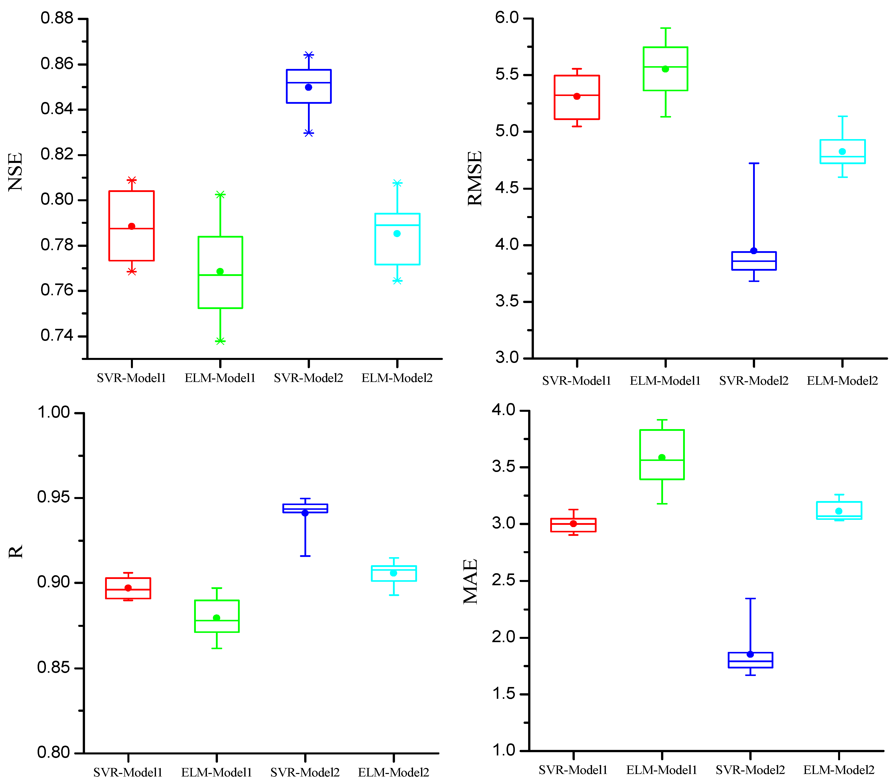
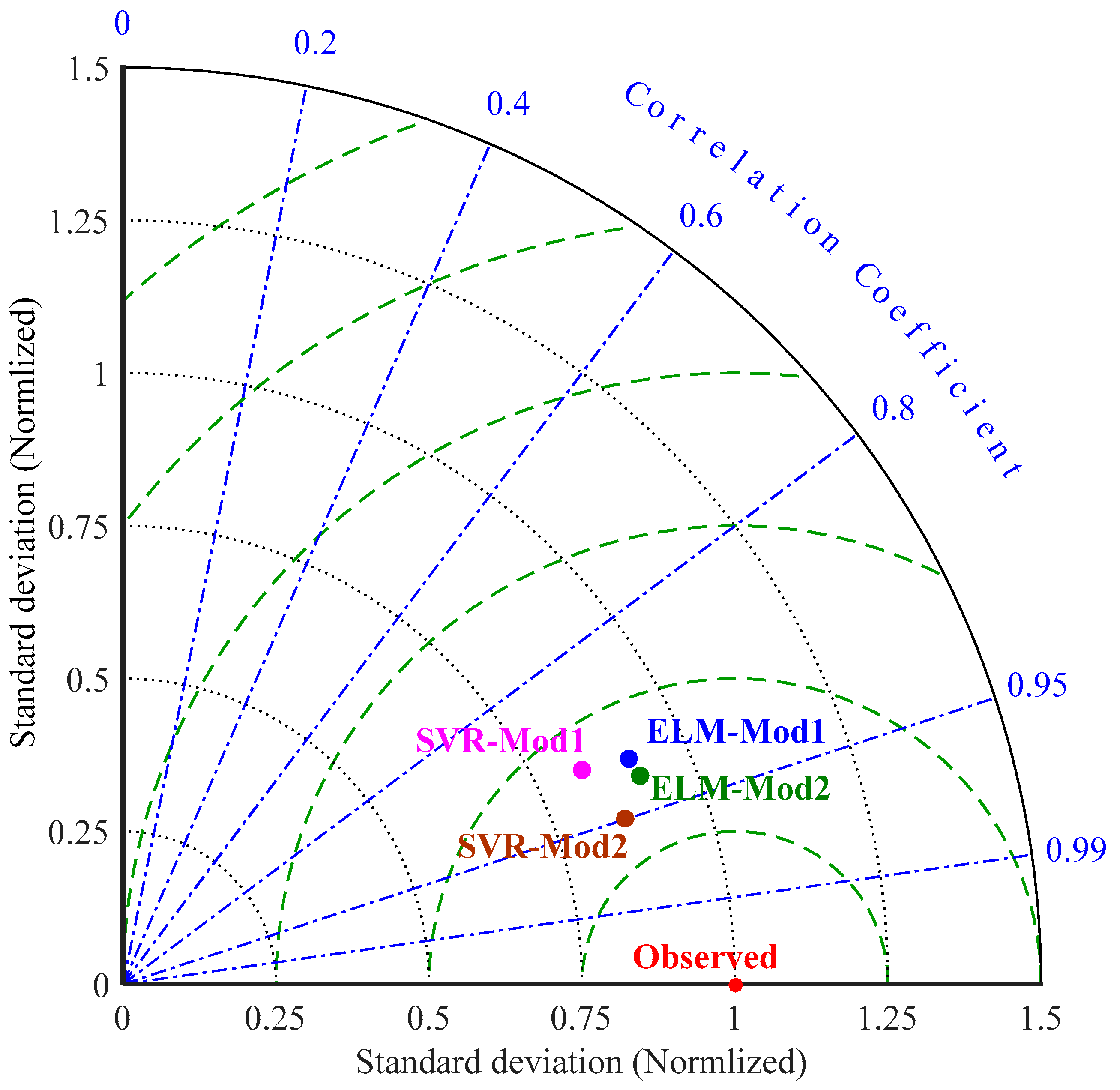
3.3. Model Simulation Calibration and Comparison

NSE, R, RMSE, and MAE were chosen as the criteria to verify the projection performance of the two methods. Figure 7 shows the results of the four performance criteria for the streamflow simulated by SVR and ELM. For the SVR and ELM and input combination, the R and NSE values were all above 0.88 and 0.74, respectively, the RMSE and MAE values were all below 6 mm/month and 4 mm/month, respectively, which indicated that the simulated streamflow could represent the observed streamflow in the upper watershed of the Heihe River with satisfying performances. However, when comparing the individual performances of the four criteria and simulation model combinations, we can easily see that the SVR directly using the GCM outputs had a distinctively higher performance than the other three combinations with NSE value above 0.83, R value above 0.91, RMSE value below 5 mm/month, and MAE value below 2.5 mm/month for the eight GCMs.

To comprehensively evaluate the performance of the hydrological responses simulated with the GCM inputs and using the SVR and ELM methods, we selected the Taylor diagram to depict the performances of the model results. The Taylor diagram provides a graphical framework that compares the simulations to reference data, which is the historically observed monthly streamflow. This gives a concise statistical summary of how closely the simulations match the references in terms of their correlations, root-mean-square differences, and the ratio of their variances, as an efficient measurement for evaluating multiple aspects of models and gauging the relative skill of many different models [45,46]. Figure 8 describes the streamflow performance derived from the downscaled precipitation and temperature series (Model 1) and the ensemble of GCM output predictors (Model 2). The SVR (Model 2) showed a comparably higher performance than the other three combinations with a closer location to the observed streamflow target. This indicates that directly using GCM output variables as input for SVR can reduce intermediate downscaling links between variables and can decrease the cumulative effect of bias in the projection of future hydrological responses.

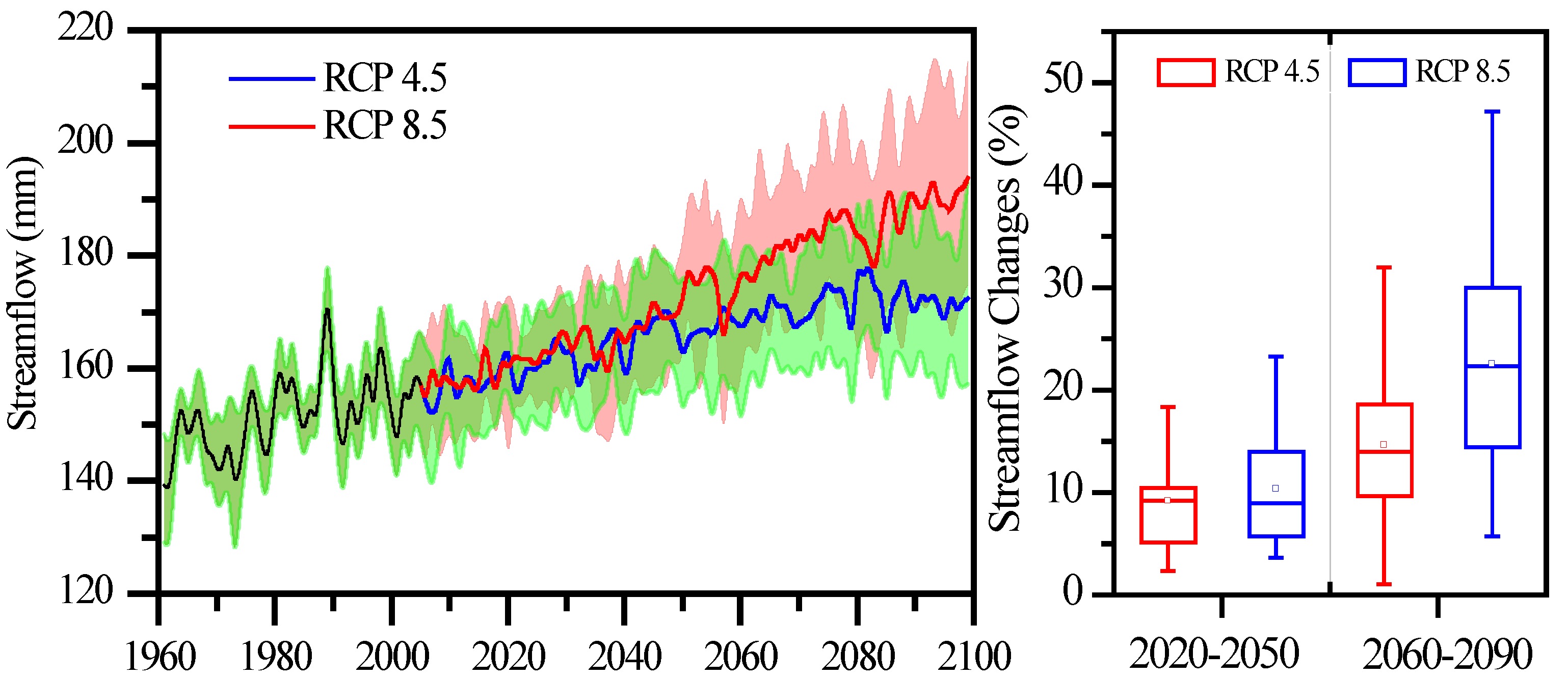
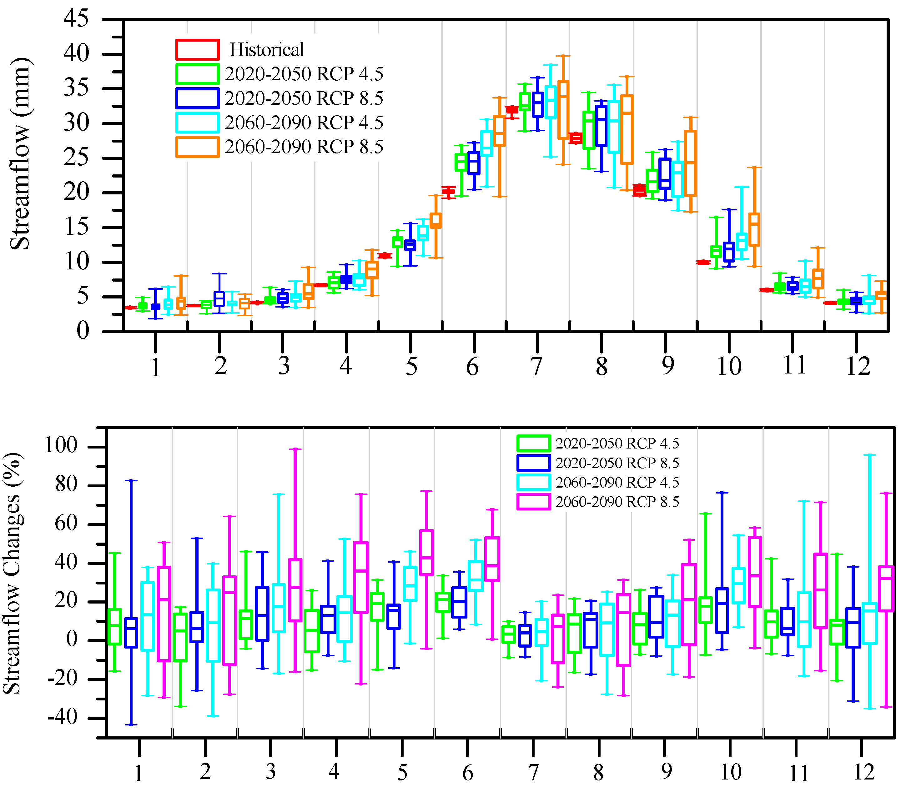
3.4. Future Streamflow Forecasting

Based on the above evaluation results, we selected the SVR with the ensemble of GCM predictors as inputs to project the future streamflow in the upper watershed of the Heihe River. We can see that the projected streamflow will continuously increase in the future with larger uncertainty when compared with precipitation and temperature (Figure 9). In the near (long) term, the average streamflow was predicted to be 156 (167) mm and 158 (182) mm under RCP scenarios 4.5 and 8.5, respectively. The distribution of the future monthly streamflow did not change compared with the historical streamflow distribution. However, the uncertainty of the predicted streamflow increased with the lengthening of data time series (Figure 10). Moreover, the uncertainty under RCP scenario 8.5 was greater than that under RCP scenario 4.5. The future summer (June, July, and August) streamflow accounts for over 50% of the annual streamflow, while the winter (December, January, and February) streamflow occupies less than 10%. It should be noted that the autumn and winter streamflow are higher in the near term than in the long term, and this phenomenon is more obvious under RCP 8.5 and has more pronounced uncertainty.

The annual streamflow will increase by 9.5% and 9.0% in the near term under RCP scenarios 4.5 and 8.5, respectively, with respect to the historical period. In the long term, the annual streamflow will increase by 13.5% and 22.0% under RCP scenarios 4.5 and 8.5, respectively, with a continuous increase in uncertainty (Figure 9). The monthly streamflow percentage changes in different periods show large variation and uncertainty. The median changes of streamflow in different months all present increasing trends. The smallest changes in streamflow occur in July with median rates of 3.18% and 3.70% in the near term and 4.64% and 3.66% in the long term under RCP scenarios 4.5 and 8.5, respectively. Meanwhile, the uncertainty in July is also the smallest when compared to the other months. The months with most increasing in streamflow are May, June, and October, and the streamflow increase is more pronounced in the long term (2060–2090) under RCP scenario 8.5. From the Sen Slope results (

Table 3. Median future slope change from the results of Sen Slope assessment (mm/yr).

Streamflow Changes	RCP 4.5		RCP 8.5
	2020–2050	2060–2090	2020–2050	2060–2090
Spring (MAM)	0.13 **	0.08 *	0.1 **	0.11 *
Summer (JJA)	0.08	0.02	0.16 **	0.13 *
Autumn (SON)	0.03	0.03	0.15 **	0.1 *
Winter (DJF)	0.04 **	0.03	0.01	0.02
Annual	0.29 **	0.14 *	0.30 **	0.43 **

Note: * represents significance at p < 0.05, ** represents significance at p < 0.01.

), we can see the changes in spring streamflow are more significant than those in the other three seasons under RCP scenario 4.5. However, under RCP scenario 8.5, the changes are all significant in all seasons except winter. Annually, in the near term, the trends of streamflow are similar under the two scenarios, while in the long term, the trend of streamflow is three times larger under RCP scenario 8.5 than under 4.5.

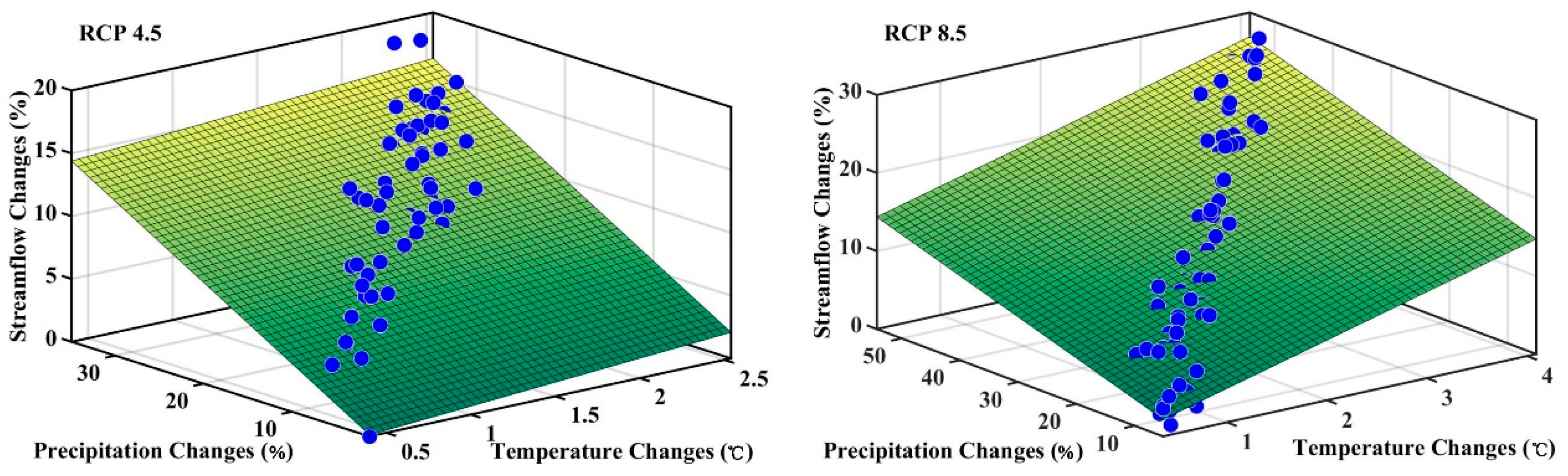
3.5. Future Climate Change Impact on the Water Yield

In order to investigate the hydrological response sensitivity to future precipitation and temperature anomaly, we averaged the SVR simulated annual streamflow, precipitation, and temperature derived by the ensemble GCMs from 1961 to 2099. The annual changes in streamflow (R, %), precipitation (P, %), and temperature (T, °C) were calculated with respect to the historical period (1961–2005). Figure 11 shows scatter plots of the simulated streamflow variation responses to precipitation and temperature changes and the fitting surface of a linear equation with two variables under two scenarios. The fitting equations are

$$\mathrm{For}\mathrm{RCP}4.5:\Delta \mathrm{R}=0.913\Delta \mathrm{T}+0.423\Delta \mathrm{P}-0.759p<0.05$$

(14)

$$\mathrm{For}\mathrm{RCP}8.5:\Delta \mathrm{R}=3.366\Delta \mathrm{T}+0.247\Delta \mathrm{P}-0.309p<0.05$$

(15)

The fitting expressions show a positive relation between streamflow variation and temperature and precipitation changes. That is to say, the streamflow is predicted to increase along with the increases in temperature and precipitation. Comparing the streamflow response equation under two scenarios, for a 1 °C increase in temperature and no change in precipitation, the streamflow is predicted to increase much more under RCP scenario 8.5 than under scenario 4.5, which means that the temperature is more sensitive to the steamflow change under RCP 8.5. For a 1% increase in precipitation and no change in temperature, the streamflow is predicted to increase more under RCP scenario 4.5 than under scenario 8.5, which means that precipitation is more sensitive to steamflow changes under RCP 4.5.

4. Discussion and Summary

The prediction of future hydrological responses is related to the GCM outputs, the length of the predicted time period, the bias correction method used, and the climate change scenario [47]. In this study, we employed eight GCMs and two artificial-intelligence-based methods to assess the future streamflow response to future climate change in a mountainous watershed in northwest China. Based on the results the machine-learning-based SVR and ELM methods showed very good performances in the projection of future hydrological responses. Machine learning algorithms provide an explanation of an externally driven process without the need for complex physical models [48]. Ease of experimentation, simple yet fast training and testing phases, and low computational burden are some advantages of using AI techniques [23]. In addition, the inputs of machine-learning-based methods can be optional: Normally the more inputs relative to the predictand, the better the forecast performance. In contrast, the inputs of physical models are fixed and are usually limited by the downscaling of GCMs with a cumulative error effect, which leads to poor simulation results. It is noteworthy that the two AI-based models showed that the SVR model was more robust with a better ability to downscale the GCM data compared with the ELM model. Without considering the internal physical connection between hydrological components and climatic variables, the methods presented in this paper can project local hydrological responses by building on the appropriate statistical relationships between the observed targets and the surface–atmospheric features.

There are inevitable sources of uncertainty in the prediction of future hydrological responses using GCM outputs, such as the uncertainty from the GCM structure, different inputs from atmospheric variables, and the forcing condition. In addition, the uncertainty derived from the different GCM outputs is a prime source of a physical model’s fidelity. Thus, multiple GCM outputs should be considered in the projection of regional climatic properties. In this study, the eight GCM outputs showed very close historical hydrological hindcasting performance and were consistent with the targets, but the future hydrological projections contained great uncertainty. In this regard, many GCM selections, simulation methods, and warming scenarios and trajectories are considered invaluable tools for advancing the relevance of hydrological responses to give more meaningful local-scale applications. Using the GCM output variable as an input for SVR can reduce intermediate downscaling links between variables and decrease the cumulative effect of bias in the projection of future hydrological responses.

Future temperature and precipitation in the study area will increase in the future under both scenarios, and the increase is more pronounced under RCP scenario 8.5 than under scenario 4.5. Future streamflow is affected by the regional precipitation and temperature, showing an increase in the near term (2020–2050) and long term (2060–2090) when compared with the historical period (1961–2005). Temperature was shown to be more sensitive to the streamflow change under RCP 8.5, while precipitation was shown to be more sensitive to the streamflow change under RCP 4.5. The implications of these results may provide water resource managers with the tools to implement water planning policy and adaptation strategies for climate change in the region.

References

1. IPCC. Climate Change 2014: Synthesis Report; Contribution of Working Groups I, II and III to the Fifth Assessment Report of the Intergovernmental Panel on Climate Change; IPCC: Geneva, Switzerland, 2014; p. 151. [Google Scholar]
2. Sunde, M.G.; He, H.S.; Hubbart, J.A.; Urban, M.A. Integrating downscaled CMIP5 data with a physically based hydrologic model to estimate potential climate change impacts on streamflow processes in a mixed-use watershed. Hydrol. Process. 2017, 31, 1790–1803. [Google Scholar] [CrossRef]
3. Wagena, M.B.; Sommerlot, A.; Abiy, A.Z.; Collick, A.S.; Langan, S.; Fuka, D.R.; Easton, Z.M. Climate change in the Blue Nile Basin Ethiopia: Implications for water resources and sediment transport. Clim. Chang. 2016, 139, 229–243. [Google Scholar] [CrossRef]
4. Thompson, J.R.; Green, A.J.; Kingston, D.G. Potential evapotranspiration-related uncertainty in climate change impacts on river flow: An assessment for the Mekong River basin. J. Hydrol. 2014, 510, 259–279. [Google Scholar] [CrossRef] [Green Version]
5. Guo, Y.; Shen, Y. Agricultural water supply/demand changes under projected future climate change in the arid region of northwestern China. J. Hydrol. 2016, 540, 257–273. [Google Scholar] [CrossRef]
6. Chen, H.; Xu, C.-Y.; Guo, S. Comparison and evaluation of multiple GCMs, statistical downscaling and hydrological models in the study of climate change impacts on runoff. J. Hydrol. 2012, 434, 36–45. [Google Scholar] [CrossRef]
7. Reshmidevi, T.V.; Nagesh Kumar, D.; Mehrotra, R.; Sharma, A. Estimation of the climate change impact on a catchment water balance using an ensemble of GCMs. J. Hydrol. 2018, 556, 1192–1204. [Google Scholar] [CrossRef] [Green Version]
8. Ghosh, K.G. Analysis of Rainfall Trends and its Spatial Patterns During the Last Century over the Gangetic West Bengal, Eastern India. J. Geovis. Spat. Anal. 2018, 2, 15. [Google Scholar] [CrossRef]
9. Olabode, O.F. Potential Groundwater Recharge Sites Mapping in a Typical Basement Terrain: A GIS Methodology Approach. J. Geovis. Spat. Anal. 2019, 3, 5. [Google Scholar] [CrossRef]
10. Asong, Z.E.; Khaliq, M.N.; Wheater, H.S. Projected changes in precipitation and temperature over the Canadian Prairie Provinces using the Generalized Linear Model statistical downscaling approach. J. Hydrol. 2016, 539, 429–446. [Google Scholar] [CrossRef]
11. Salvi, K.; Kannan, S.; Ghosh, S. High-resolution multisite daily rainfall projections in India with statistical downscaling for climate change impacts assessment. J. Geophys. Res. Atmos. 2013, 118, 3557–3578. [Google Scholar] [CrossRef]
12. Kouhestani, S.; Eslamian, S.S.; Abedi-Koupai, J.; Besalatpour, A.A. Projection of climate change impacts on precipitation using soft-computing techniques: A case study in Zayandeh-rud Basin, Iran. Glob. Planet. Chang. 2016, 144, 158–170. [Google Scholar] [CrossRef]
13. Chen, S.-T.; Yu, P.-S.; Tang, Y.-H. Statistical downscaling of daily precipitation using support vector machines and multivariate analysis. J. Hydrol. 2010, 385, 13–22. [Google Scholar] [CrossRef]
14. Sehgal, V.; Lakhanpal, A.; Maheswaran, R.; Khosa, R.; Sridhar, V. Application of multi-scale wavelet entropy and multi-resolution Volterra models for climatic downscaling. J. Hydrol. 2018, 556, 1078–1095. [Google Scholar] [CrossRef]
15. Mehrotra, R.; Sharma, A.; Nagesh Kumar, D.; Reshmidevi, T.V. Assessing future rainfall projections using multiple GCMs and a multi-site stochastic downscaling model. J. Hydrol. 2013, 488, 84–100. [Google Scholar] [CrossRef]
16. Wilby, R.L.; Dawson, C.W. The Statistical DownScaling Model: Insights from one decade of application. Int. J. Climatol. 2013, 33, 1707–1719. [Google Scholar] [CrossRef]
17. Musau, J.; Sang, J.; Gathenya, J.; Luedeling, E. Hydrological responses to climate change in Mt. Elgon watersheds. J. Hydrol. Reg. Stud. 2015, 3, 233–246. [Google Scholar] [CrossRef] [Green Version]
18. Birkinshaw, S.J.; Guerreiro, S.B.; Nicholson, A.; Liang, Q.; Quinn, P.; Zhang, L.; He, B.; Yin, J.; Fowler, H.J. Climate change impacts on Yangtze River discharge at the Three Gorges Dam. Hydrol. Earth Syst. Sci. 2017, 21, 1911–1927. [Google Scholar] [CrossRef] [Green Version]
19. Zhang, Y.; Fu, G.; Sun, B.; Zhang, S.; Men, B. Simulation and classification of the impacts of projected climate change on flow regimes in the arid Hexi Corridor of Northwest China. J. Geophys. Res. Atmos. 2015, 120, 7429–7453. [Google Scholar] [CrossRef]
20. Wang, W.; Xing, W.; Shao, Q. How large are uncertainties in future projection of reference evapotranspiration through different approaches? J. Hydrol. 2015, 524, 696–700. [Google Scholar] [CrossRef]
21. Deo, R.C.; Şahin, M. Application of the extreme learning machine algorithm for the prediction of monthly Effective Drought Index in eastern Australia. Atmos. Res. 2015, 153, 512–525. [Google Scholar] [CrossRef] [Green Version]
22. Sarhadi, A.; Burn, D.H.; Yang, G.; Ghodsi, A. Advances in projection of climate change impacts using supervised nonlinear dimensionality reduction techniques. Clim. Dyn. 2017, 48, 1329–1351. [Google Scholar] [CrossRef]
23. Sarhadi, A.; Burn, D.H.; Johnson, F.; Mehrotra, R.; Sharma, A. Water resources climate change projections using supervised nonlinear and multivariate soft computing techniques. J. Hydrol. 2016, 536, 119–132. [Google Scholar] [CrossRef] [Green Version]
24. Srinivas, V.V.; Basu, B.; Nagesh Kumar, D.; Jain, S.K. Multi-site downscaling of maximum and minimum daily temperature using support vector machine. Int. J. Climatol. 2014, 34, 1538–1560. [Google Scholar] [CrossRef]
25. Su, B.; Zeng, X.; Zhai, J.; Wang, Y.; Li, X. Projected precipitation and streamflow under SRES and RCP emission scenarios in the Songhuajiang River basin, China. Quat. Int. 2015, 380–381, 95–105. [Google Scholar] [CrossRef]
26. Huang, G.-B. What are Extreme Learning Machines? Filling the Gap Between Frank Rosenblatt’s Dream and John von Neumann’s Puzzle. Cogn. Comput. 2015, 7, 263–278. [Google Scholar] [CrossRef]
27. Duhan, D.; Pandey, A. Statistical downscaling of temperature using three techniques in the Tons River basin in Central India. Theor. Appl. Climatol. 2015, 121, 605–622. [Google Scholar] [CrossRef]
28. Yin, Z.; Feng, Q.; Yang, L.; Deo, C.R.; Wen, X.; Si, J.; Xiao, S. Future Projection with an Extreme-Learning Machine and Support Vector Regression of Reference Evapotranspiration in a Mountainous Inland Watershed in North-West China. Water 2017, 9, 880. [Google Scholar] [CrossRef]
29. Yin, Z.; Feng, Q.; Yang, L.; Wen, X.; Si, J.; Zou, S. Long Term Quantification of Climate and Land Cover Change Impacts on Streamflow in an Alpine River Catchment, Northwestern China. Sustainability 2017, 9, 1278. [Google Scholar] [CrossRef]
30. Yang, L.; Feng, Q.; Yin, Z.; Wen, X.; Si, J.; Li, C.; Deo, R.C. Identifying separate impacts of climate and land use/cover change on hydrological processes in upper stream of Heihe River, Northwest China. Hydrol. Process. 2017, 31, 1100–1112. [Google Scholar] [CrossRef]
31. Taylor, K.E.; Stouffer, R.J.; Meehl, G.A. An Overview of CMIP5 and the Experiment Design. Bull. Am. Meteorol. Soc. 2012, 93, 485–498. [Google Scholar] [CrossRef] [Green Version]
32. Collier, M.; Uhe, P. CMIP5 Datasets from the ACCESS1.0 and ACCESS1.3 Coupled Climate Models; The Centre for Australian Weather and Climate Research: Aspendale, Australia, 2012; pp. 1–32. [Google Scholar]
33. Wu, T.; Li, W.; Ji, J.; Xin, X.; Li, L.; Wang, Z.; Zhang, Y.; Li, J.; Zhang, F.; Wei, M.; et al. Global carbon budgets simulated by the Beijing Climate Center Climate System Model for the last century. J. Geophys. Res. Atmos. 2013, 118, 4326–4347. [Google Scholar] [CrossRef]
34. Liu, X.; Wu, T.; Yang, S.; Jie, W.; Nie, S.; Li, Q.; Cheng, Y.; Liang, X. Performance of the seasonal forecasting of the Asian summer monsoon by BCC_CSM1.1(m). Adv. Atmos. Sci. 2015, 32, 1156–1172. [Google Scholar] [CrossRef]
35. Voldoire, A.; Sanchez-Gomez, E.; Salas y Mélia, D.; Decharme, B.; Cassou, C.; Sénési, S.; Valcke, S.; Beau, I.; Alias, A.; Chevallier, M.; et al. The CNRM-CM5.1 global climate model: Description and basic evaluation. Clim. Dyn. 2013, 40, 2091–2121. [Google Scholar] [CrossRef]
36. Martin, G.M.; Bellouin, N.; Collins, W.J.; Culverwell, I.D.; Halloran, P.R.; Hardiman, S.C.; Hinton, T.J.; Jones, C.D.; McDonald, R.E.; McLaren, A.J.; et al. The HadGEM2 family of Met Office Unified Model climate configurations. Geosci. Model Dev. 2011, 4, 723–757. [Google Scholar] [CrossRef] [Green Version]
37. Watanabe, M.; Suzuki, T.; O’ishi, R.; Komuro, Y.; Watanabe, S.; Emori, S.; Takemura, T.; Chikira, M.; Ogura, T.; Sekiguchi, M.; et al. Improved Climate Simulation by MIROC5: Mean States, Variability, and Climate Sensitivity. J. Clim. 2010, 23, 6312–6335. [Google Scholar] [CrossRef]
38. Yukimoto, S.; Adachi, Y.; Hosaka, M.; Sakami, T.; Yoshimura, H.; Hirabara, M.; Tanaka, T.Y.; Shindo, E.; Tsujino, H.; Deushi, M.; et al. A New Global Climate Model of the Meteorological Research Institute: MRI-CGCM3—Model Description and Basic Performance—. J. Meteorol. Soc. Jpn. Ser. II 2012, 90, 23–64. [Google Scholar] [CrossRef]
39. Huang, G.-B.; Chen, L. Convex incremental extreme learning machine. Neurocomputing 2007, 70, 3056–3062. [Google Scholar] [CrossRef]
40. Huang, G.-B.; Zhu, Q.-Y.; Siew, C.-K. Extreme learning machine: Theory and applications. Neurocomputing 2006, 70, 489–501. [Google Scholar] [CrossRef]
41. Abdullah, S.S.; Malek, M.A.; Abdullah, N.S.; Kisi, O.; Yap, K.S. Extreme Learning Machines: A new approach for prediction of reference evapotranspiration. J. Hydrol. 2015, 527, 184–195. [Google Scholar] [CrossRef]
42. Gocic, M.; Petković, D.; Shamshirband, S.; Kamsin, A. Comparative analysis of reference evapotranspiration equations modelling by extreme learning machine. Comput. Electron. Agric. 2016, 127, 56–63. [Google Scholar] [CrossRef]
43. Patil, A.P.; Deka, P.C. An extreme learning machine approach for modeling evapotranspiration using extrinsic inputs. Comput. Electron. Agric. 2016, 121, 385–392. [Google Scholar] [CrossRef]
44. Yang, L.; Feng, Q.; Li, C.; Si, J.; Wen, X.; Yin, Z. Detecting climate variability impacts on reference and actual evapotranspiration in the Taohe River Basin, NW China. Hydrol. Res. 2016, 48, 596–612. [Google Scholar] [CrossRef]
45. Taylor, M.; Kosmopoulos, P.G.; Kazadzis, S.; Keramitsoglou, I.; Kiranoudis, C.T. Neural network radiative transfer solvers for the generation of high resolution solar irradiance spectra parameterized by cloud and aerosol parameters. J. Quant. Spectrosc. Radiat. Transf. 2016, 168, 176–192. [Google Scholar] [CrossRef]
46. Taylor, K.E. Summarizing multiple aspects of model performance in a single diagram. J. Geophys. Res. Atmos. 2001, 106, 7183–7192. [Google Scholar] [CrossRef]
47. Al Aamery, N.; Fox, J.F.; Snyder, M. Evaluation of climate modeling factors impacting the variance of streamflow. J. Hydrol. 2016, 542, 125–142. [Google Scholar] [CrossRef]
48. Sachindra, D.A.; Huang, F.; Barton, A.; Perera, B.J.C. Least square support vector and multi-linear regression for statistically downscaling general circulation model outputs to catchment streamflows. Int. J. Climatol. 2013, 33, 1087–1106. [Google Scholar] [CrossRef]
Figure 1. Location of the study area in China and the distribution of gauging stations.
Water 11 01588 g001
Figure 2. Schematic diagrams for future hydrological response projection.
Water 11 01588 g002
Figure 3. Performances of the Support Vector Regression (SVR) and Extreme Learning Machine (ELM) for the determination of the climate–hydrological relationship derived from the observed precipitation, temperature, and streamflow with time lag.
Water 11 01588 g003
Figure 4. Annual temperature and precipitation variation derived from the ensemble of General Circulation Models (GCM) scenarios in the upper watershed of the Heihe River. The shadows and solid lines of the left panel represent the 90% predictive uncertainty and average value, respectively. In the box plot (right panel), the dot represents the average value and the upper and lower hinges represent the 75th and 25th percentiles, respectively. The whiskers show the other data points, except for the outliers. The line within the box shows the median.
Water 11 01588 g004
Figure 5. Future change tendency for the monthly temperature at different periods and under different climate scenarios. The term “Temp” represents temperature. The red line shows the median; the borderline represents 90% predictive uncertainty.
Water 11 01588 g005
Figure 6. Future change tendency for the monthly precipitation in different periods and climate scenarios. The term “Precip.” represents precipitation. The red line shows the median; the borderline represents the 90% predictive uncertainty.
Water 11 01588 g006
Figure 7. Box plots of historical streamflow hindcast performances of SVR and ELM derived from the selected eight GCMs. The dot represents the average value, the upper and lower hinges represent the 75th and 25th percentiles, respectively. The whiskers show the other data points, except for the outliers. The line within the box shows the median.
Water 11 01588 g007
Figure 8. Taylor diagrams for depicting the standard deviation and correlation of the streamflow projected from the ensemble of General Circulation Models (GCMs) using the SVR and ELM methods. Mod1 denotes Model1, Mod2 denotes Model2.
Water 11 01588 g008
Figure 9. Annual streamflow variation under future climate change scenarios in the upper watershed of the Heihe River. The shadows and solid lines of the left panel represent the 90% predictive uncertainty and average value, respectively. In the box plot (right panel), the dot represents the average value, the upper and lower hinges represent the 75th and 25th percentiles, respectively. The whiskers show the other data points, except for the outliers. The line within the box shows the median.
Water 11 01588 g009
Figure 10. Monthly streamflow and percentage change relative to 1961–2005 under RCP scenarios 4.5 and 8.5. In the box plot, the upper and lower hinges represent the 75th and 25th percentiles, respectively. The whiskers show the other data points, except for the outliers. The line within the box shows the median.
Water 11 01588 g010
Figure 11. Streamflow variation in the experiment on the future precipitation and temperature changes under RCP scenarios 4.5 and 8.5.
Water 11 01588 g011