Biased Estimation of Groundwater Velocity from a Push-Pull Tracer Test Due to Plume Density and Pumping Rate


1
Department of Civil Engineering and Environmental Sciences, Korea Military Academy, Seoul 01805, Korea
2
School of Earth and Environmental Sciences, Seoul National University, Seoul 08826, Korea
*
Author to whom correspondence should be addressed.
Water 2019, 11(8), 1558; https://doi.org/10.3390/w11081558
Submission received: 17 June 2019
/
Revised: 19 July 2019
/
Accepted: 24 July 2019
/
Published: 28 July 2019
(This article belongs to the Section Hydrology)
Abstract
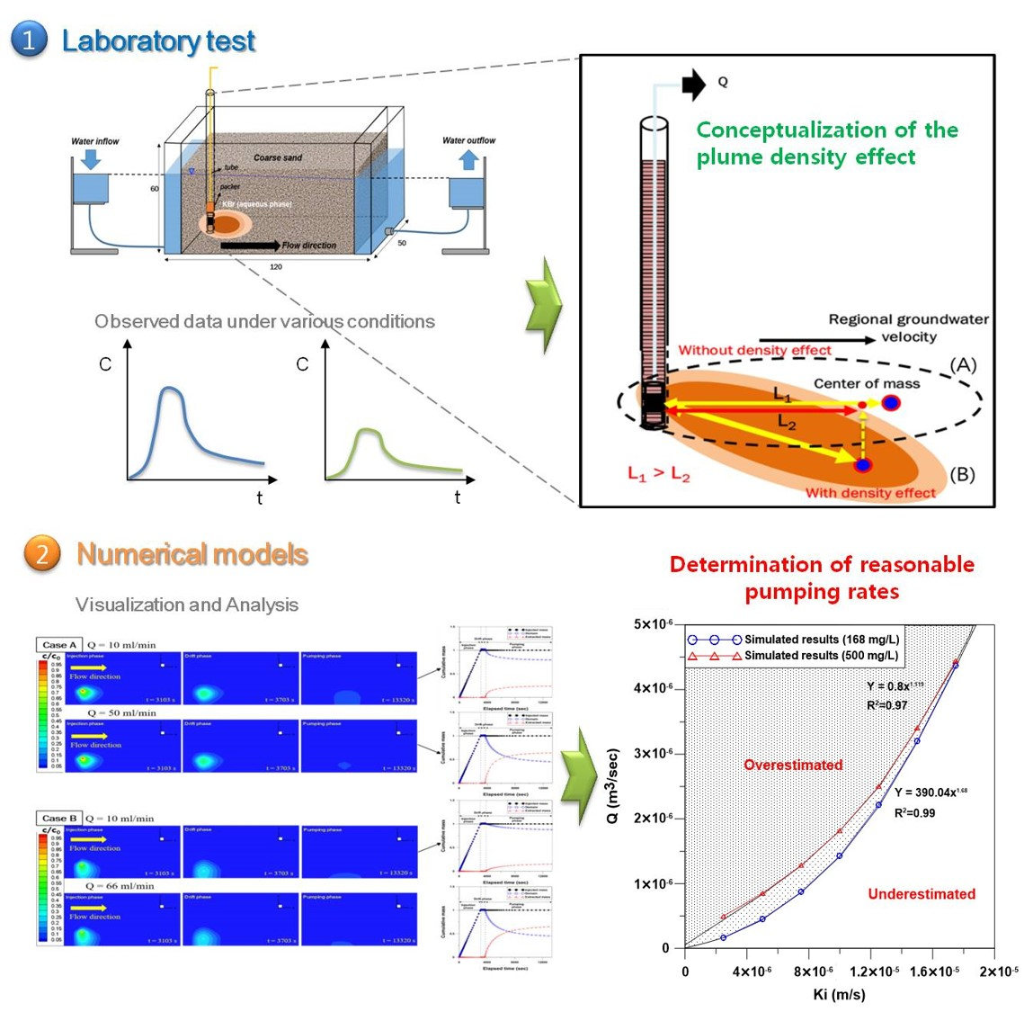
:The single-well push-pull tracer test is a convenient and cost-effective tool to estimate hydrogeological properties of a subsurface aquifer system. However, it has a limitation that test results can be affected by various experimental designs. In this study, a series of laboratory-scale push-pull tracer tests were conducted under various conditions controlling input tracer density, pumping rate, drift time, and hydraulic gradient. Based on the laboratory test results, numerical simulations were performed to evaluate the effects of density-induced plume sinking and pumping rate on the proper estimation of groundwater background linear velocity. Laboratory tests and numerical simulations indicated that the actual linear velocity was underestimated for the higher concentration of the input tracer because solute travel distance and direction during drift time were dominantly affected by the plume density. During the pulling phase, reasonable pumping rates were needed to extract the majority of injected tracer mass to obtain a genuine center of mass time (tcom). This study presents a graph showing reasonable pumping rates for different combinations of plume density and background groundwater velocity. The results indicate that careful consideration must be given to the design and interpretation of push-pull tracer tests.

1. Introduction
One of the commonly utilized methods to estimate aquifer hydrogeologic properties is a tracer test, in which nonreactive or reactive tracers are injected into a borehole to generate a breakthrough curve of the injected tracer transporting through the aquifer medium [1,2,3]. Based on the analysis of the obtained breakthrough curves from the tracer test, information about the aquifer geometry, solute transport dynamics, microbial processes, and reactive movement of the tracer can be evaluated [4,5,6,7].
Among various types of tracer test, the single-well push-pull test is a method of easy performance and no more logistical complexity with a modest cost and has been applied to estimate physical parameters such as longitudinal dispersivity, groundwater velocity, and effective porosity of the tested aquifer [8,9,10,11,12]. The push-pull test consists of three phases. The first step is the injection phase (so-called “push”). In this step, a prepared solution is injected into the aquifer at an injection well. The second step is the drift phase, where the injected solution moves along with the ambient groundwater flow. The final step is the pumping phase (so-called “pull”), where the injected solution is pumped back toward the same well as is used for injection. Meigs and Beauheim [13] presented applications of single-well injection/withdrawal and multi-well convergent tracer tests to evaluate advective and diffusive transport processes in porous media. Leap and Kaplan [14] and Hall et al. [15] used tracer tests to analyze the arrival time of the center of mass from the tracer breakthrough curve and obtain information on groundwater velocity and effective porosity.
Although the push-pull tracer test has an advantage of being easy to perform by using only one tested borehole, hydraulic conditions of the tested field or test design of the push-pull test could cause misinterpretation of the aquifer properties. Hwang [16] performed single-well push-pull tests under different experimental conditions by changing extraction rate, drift time, hydraulic conductivity, and hydraulic gradient. Based on the test results, Hwang [16] concluded that the mass recovery rate was inversely proportional to the drift time and the hydraulic gradient. Hebig et al. [17] conducted single-well push-pull tests with different chaser volumes and found that the chaser volume could affect the main peak concentration of the breakthrough curve. Wang et al. [18] reported that single-well push-pull test results can be different in steady-state and transient flow conditions and such differences increased with the decreasing specific storage. Paradis et al. [12] considered the displacement during the injection phase, which resulted in more accurate calculation of effective porosity.
Under some hydrogeological conditions, density differences between the background fluid and solute or thermal plume can appear because of changes in solute concentration or temperature. Plumes related to seawater intrusion, high-level radioactive waste disposal, groundwater contamination, and geothermal energy production can be examples [19]. In such cases, a density-induced sinking or rising effect can appear during transport and the density-induced sinking has been discussed in transport-related studies [20,21,22,23,24,25].
The method of Hall et al. [15] was theoretically developed for a field-scale. However, it was possible to perform the push-pull test successfully on a small-scale by performing a tracer injection and extraction using simple experimental equipment, such as plastic syringes [10]. In addition, Leap and Kaplan [14] suggested the method of calculating the groundwater velocity using the push-pull test for the first time and proved the validity of the theory by lab-scale experiments. Leap and Kaplan [14] and Hall et al. [15] did not consider the effect of density-induced sinking during a drift phase and pumping rate during pumping phase, and the effect of uncertainty on groundwater velocity calculation was not taken into account. In the push-pull tracer test, the density effect can act as a major controlling factor for the drift phase and consequently biased estimation of the groundwater velocity would result. However, none of the previous studies have examined the tracer density effect on estimating linear groundwater velocity using the single-well push-pull tracer test.
The purpose of this paper is to demonstrate that the push-pull tracer test design requires consideration of density effect and pumping rate through a lab-scale push-pull tracer test and simulation. In order to achieve the purpose of the paper, the following three main contents are described: (1) assess the impact of density-induced sinking on the estimation of groundwater linear velocity using the lab-scale push-pull tracer test and simulation, (2) investigate the effect of pumping rate during the pull phase, and (3) present reasonable pumping rate estimation for different combinations of plume density and groundwater velocity.
2. Methods
2.1. Laboratory Push-Pull Tests
2.1.1. Experimental Setup and Tracer Recovery
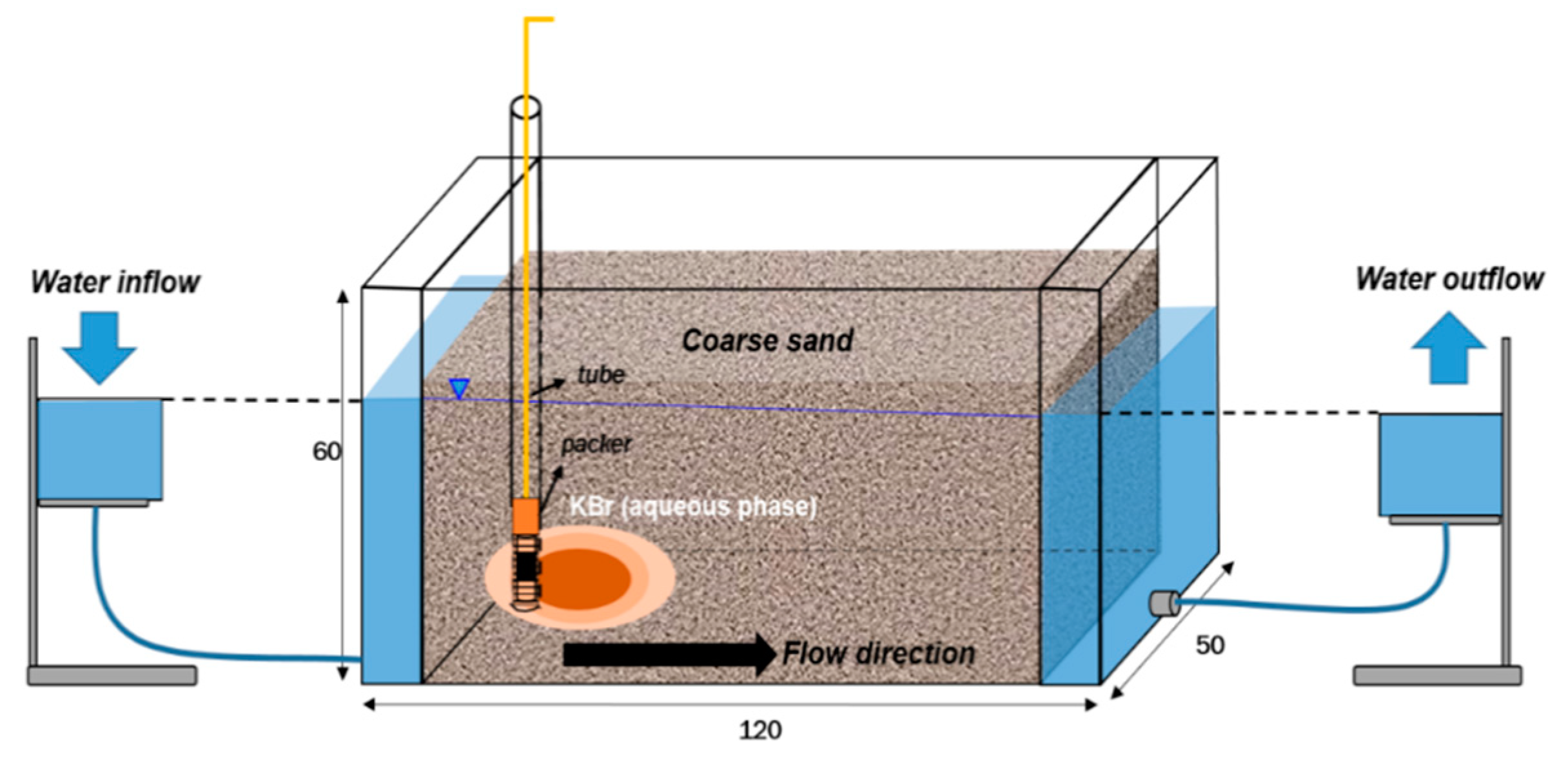
The laboratory push-pull tracer tests were performed to investigate the impacts of various density conditions of injected tracer on the pattern of breakthrough curves. The groundwater linear velocity was calculated with observed hydraulic gradient, effective porosity, and hydraulic conductivity of the experimental setup and it was considered as the real linear velocity. The linear velocity estimated from the solute breakthrough curve of the push-pull tracer test was compared with the real linear velocity to confirm the accuracy of the tracer test. Bromide (Br) was chosen as the tracer for the experiment because it is chemically conservative and nonvolatile. An acrylic glass tank was made with inner dimensions of 120 cm × 50 cm × 60 cm (length × width × height) with a thickness of 2 cm. At both sides of the tank, hydraulic heads were controlled to generate the intended hydraulic gradient for the tracer test (Figure 1). For injecting and extracting water, the test well was made of 2 mm thick acrylic pipe with an inner diameter of 2 cm. The well screen was placed at the end of the well, in which the length of the slotted interval was 5 mm. The well for injection/extraction was located at x = 15 cm and y = 10 cm, and the well end was located 10 cm above the sand tank bottom. The top of the well was strapped with aluminum frames to minimize the occurrence of the preferential pathway during filling the tank by preventing the formation of gaps between the well and the sand.
The experimental tank was carefully packed with coarse sand to prevent air trapping inside the porous medium and the groundwater linear velocity was computed using the parameters obtained from the tests described below. Hydraulic conductivity of the porous medium composed of the sand was measured by constant-head permeability tests. A total of nine permeability tests were performed and the average value was chosen as the representative value (Table 1). The porosity of the material was derived by measuring the dry soil sand volume and the bulk volume. The average porosity value of repeated measurements was 0.34. The effective porosity of the porous medium was estimated by column tests in which a 5TE sensor (DECAGON, Pullman, WA, USA) measured the soil moisture content as drainage progressed and subtracted it from saturated water content (Figure S1). The effective porosity was defined as total porosity minus field capacity. The water content was measured for 5 days after gravity drainage of the fully saturated column and the field capacity value of coarse sand was 0.02. The estimated relative effective porosity of the coarse sand is provided in Table 1.
Variable-density conditions of the tracer were applied to verify the density effect in the push-pull tracer test, as listed in Table 2. According to Barth et al. [25], 357 mg/L of potassium bromide (KBr) solution did not cause density-induced sinking, but, if the KBr concentration exceeded 357 mg/L, density-induced sinking occurred under the hydraulic gradient of . Based on the observation from Barth et al. [25], the injected concentrations of Br were determined from 168 mg/L to 2450 mg/L in the laboratory single-well push-pull tracer tests (Tests 1–4 in Table 2). We controlled the hydraulic gradient in the sand tank at 0.003 in Tests 1–4. It was the minimum hydraulic gradient that could be made under the experimental conditions. In Tests 5–7, the hydraulic gradient was controlled at 0.012 to investigate the results under a higher hydraulic gradient condition. The drift time for Tests 5–7 was adjusted to 5 min to increase the recovery amount of the injected tracer.
Tracer sampling intervals were started at 2 min and gradually increased to 30 min until the end of tests. In the early time of the pull phase, a short time interval for sampling was applied because the peak concentration of the tracer is generally detected in the early time of the test and the change of concentration also appears significantly. After the early stage, the sampling time interval became longer because a lower concentration gradient was expected at the late time of the pull phase and the change of concentration would be insignificant.
Additional laboratory tests were performed with three density conditions (no-density, 3 g/L and 6 g/L) of KBr tracer to visualize the density-induced sinking. The 1 g of food dye (red) was used to visualize the transportation and 30 mL of KBr tracer was injected at a screen point of the well (plastic tube). The injection rate was 1.25 mL/min and the hydraulic gradient of the test was 0.01. Tracer plume tracking was performed using the open-source software ImageJ [26]. It can mark the centroid of each tracer plume captured every 5 min after injection.
2.1.2. Analytical Computation of Groundwater Velocity
Based on Darcy’s law, the linear velocity from the experimental setting can be computed by,
where, V is the average linear groundwater velocity (m/s), K is the horizontal hydraulic conductivity (m/s), i is the horizontal hydraulic gradient (dimensionless), and n is the effective porosity (dimensionless).
By using the push-pull tracer test, Hall et al. [15] suggested a method to estimate linear velocity and effective porosity from the pulled tracer’s breakthrough curve. Assuming pumping during the pull phase makes a concentric capture-zone and applying Darcy’s law, Hall et al. derived the equations to compute groundwater velocity (VH) and effective porosity (ne) as follows:
where, Q is the pumping rate during the pull phase (m3/s), is the time elapsed from the start of pumping until one-half of the injected tracer is recovered (s), b is the aquifer thickness (m), and is the time elapsed from the injection of the tracer until the center of mass of the tracer, i.e., one-half of the injected tracer, is recovered by pumping (i.e., drift time plus ). From the obtained breakthrough curve from the single-well push-pull tracer test, the tcom can be obtained. It is used to determine the linear groundwater velocity and the effective porosity by using Equations (2) and (3).
2.2. Numerical Simulation
A numerical model was constructed to reproduce an analogous system with the experimental push-pull tracer test. With the numerical model, reasons for the bias of the linear groundwater velocity estimated based on the tracer tests of the linear groundwater velocity obtained from the hydraulically controlled experimental setting. In addition, different combinations of plume density and extraction rate were applied as input data to simulate their effects on the plume transport. The HydroGeoSphere modeling program [27], which can simulate the groundwater flow and the variable-density solute transport, was used in this study.
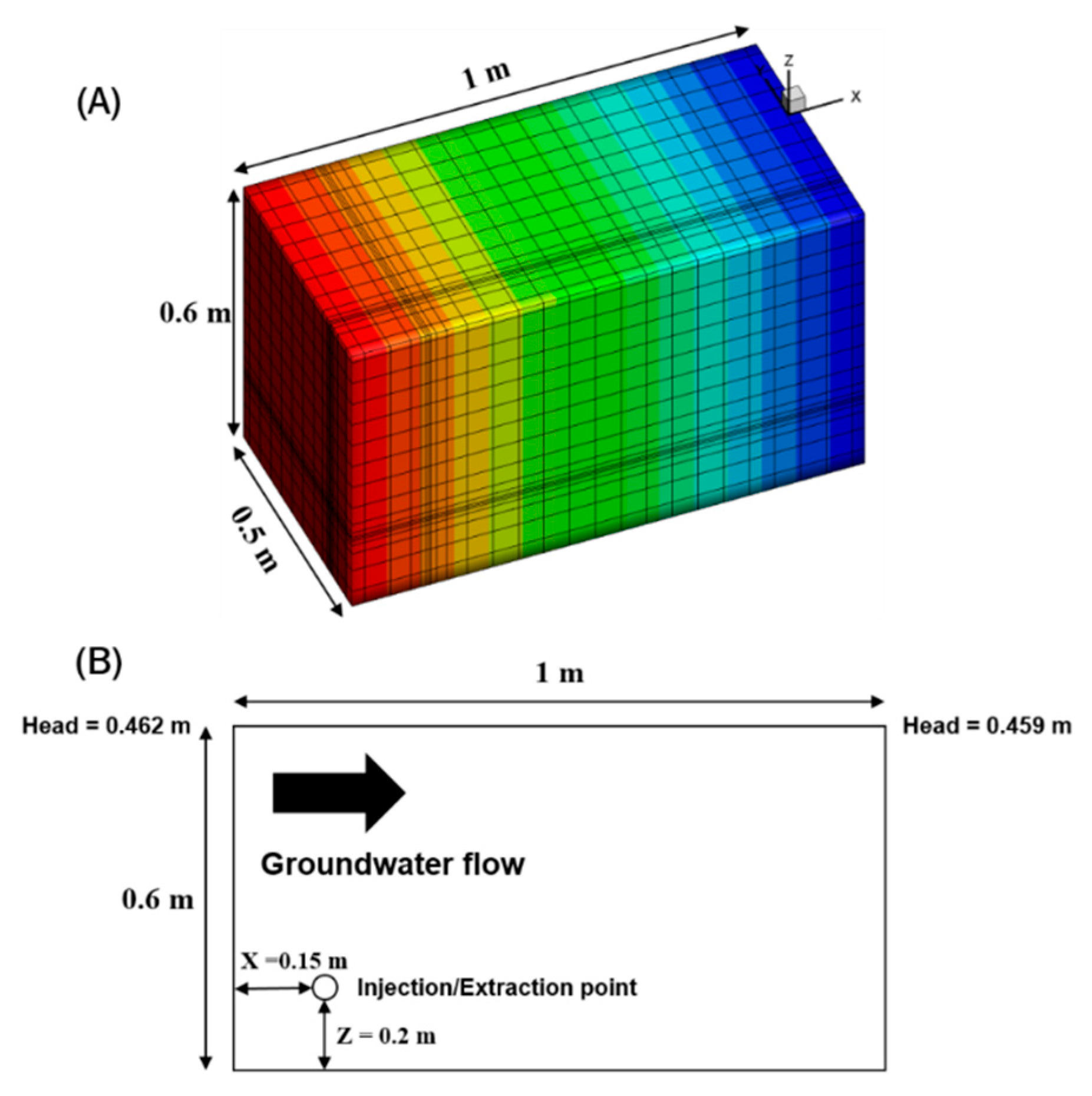
According to the settings of the sand tank experiment, a three-dimensional model domain was constructed, as shown in Figure 2. Variably sized grids were generated while finer grids were inserted near the tested well. The generated numbers of nodes and elements were 8721 and 7488, respectively. The left and right sides of the model (x = 0 m and x = 1 m) were assigned as a Dirichlet-type boundary condition to create a constant hydraulic gradient. Other boundaries were no-flow boundaries. The well node for injection and extraction after the injection was assigned at the same location as the well of the laboratory experiment, and the initial concentration of all nodes was given as . Model parameters for the numerical simulation are shown in Table 3. The hydraulic properties were estimated by laboratory test and the free-solution diffusion coefficient of KBr was given as [28].
Modeling calibration was implemented by generating the same tracer test conditions as the laboratory experiments. We determined that the model calibration was completed when the root mean square error (RMSE) of the breakthrough curve derived from the experimental breakthrough curves and simulation was less than 0.05, and the trial-and-error method was applied to adjust the dispersivity to calibrate the model.
3. Results and Discussion
3.1. Results of Laboratory Push-Pull Tracer Tests
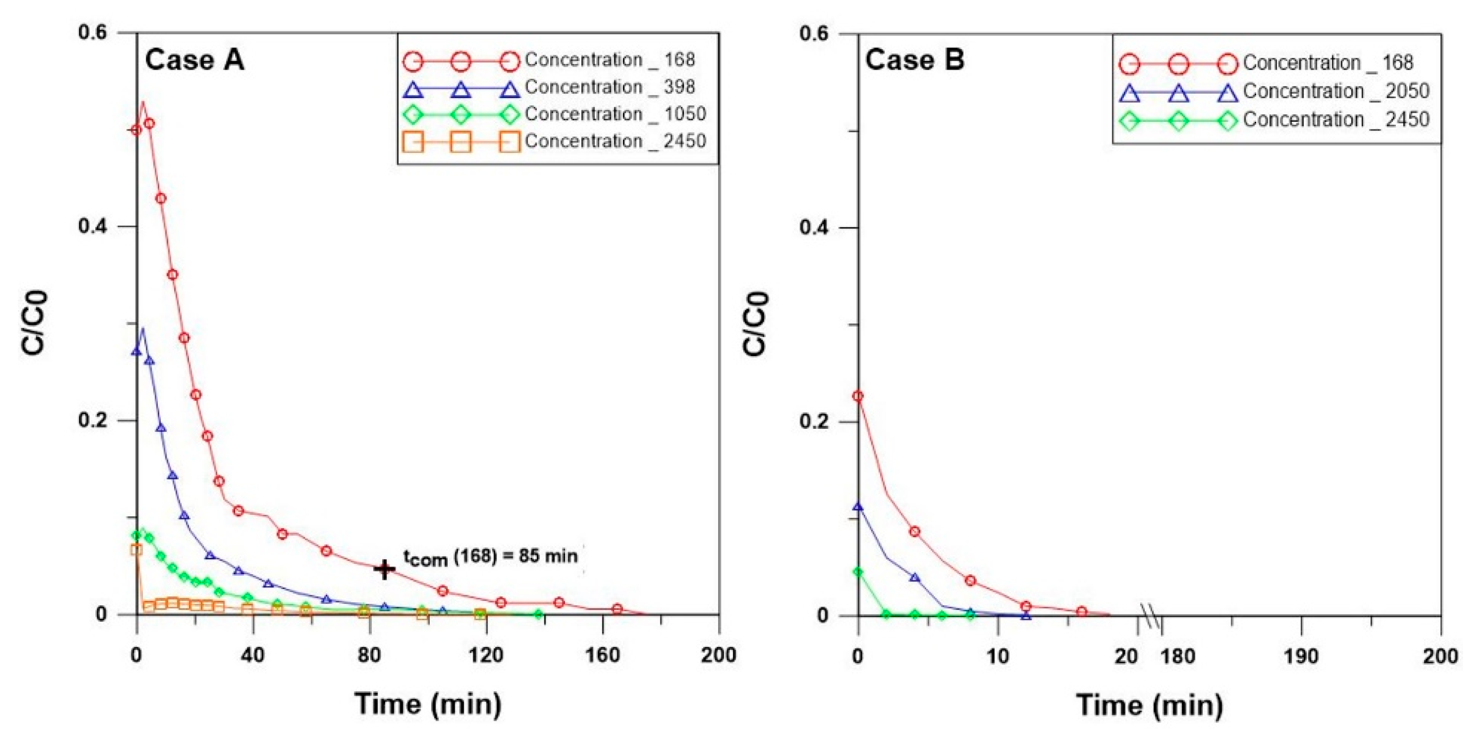
Figure 3a showed the breakthrough curves of laboratory push-pull tests under various tracer concentration values at the hydraulic gradient of 0.003 (Tests 1–4). The highest value (0.53) of pull-phase relative concentration (C/C0) appeared for the lowest tracer concentration of 168 mg/L. As the concentration of tracer increased (168 mg/L → 398 mg/L → 1050 mg/L → 2450 mg/L), the pull-phase C/C0 value decreased (0.53 → 0.29 → 0.09 → 0.07). The same tests were performed under a greater hydraulic gradient of 0.012 (Tests 5–7, Figure 3b). In this case, a decreasing trend (0.23 → 0.11 → 0.05) of the initial pull-phase C/C0 value appeared to decrease more rapidly with the increase of the tracer concentration injected for the tests (168 mg/L → 2050 mg/L → 2450 mg/L).
The primary effect that lowered the peak of the breakthrough curve with the increase in the injected tracer concentration was reasoned to be a density-induced sinking effect. Istok and Humphrey [29] investigated the density effect on the breakthrough curve from two-well tracer tests with a sandbox and C/C0 of the breakthrough curve was lowered because of the density-induced sinking effect. During the drift phase of the tests, an increase in injection tracer concentration would intensify the sinking effect of the injected solute migrating with the ambient groundwater flow. Furthermore, with the greater hydraulic gradient (0.012) in Tests 5–7, the tracer plume transported further during the shorter drifting time of Tests 1–4 and therefore, part of the tracer plume positioned beyond the bound of the capture zone for the pull phase compared with the case of the lower hydraulic gradient of 0.003.
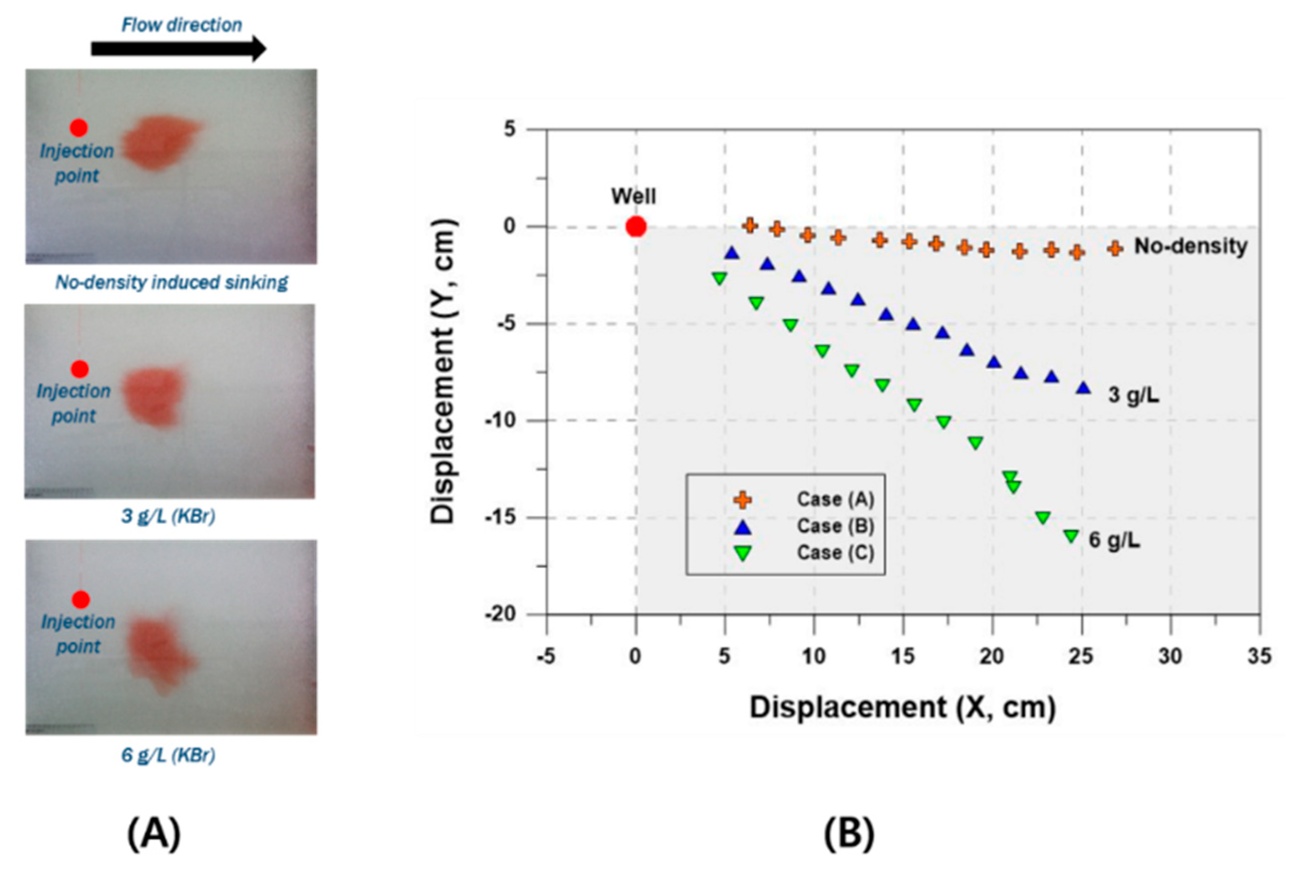
The laboratory tracer test results in Figure 4 are reasonably explained based on density-induced sinking during drift time. The denser plume (3 g/L and 6 g/L in Figure 4), compared with the plume without the density difference with the background water (no-density difference case in Figure 4), became less apart laterally from the pumping well (26.9 cm under the no-density condition, 25.1 cm under the 3 g/L condition, 24.4 cm under the 6 g/L condition). However, the pumping produced a strong lateral flow field toward the pumping well screen interval, part of the sunk plume became difficult to be transported back to the well. This could cause the lowered peak concentration in the test case with higher initial tracer injection concentration. As a result, a breakthrough curve showing a shorter tracer recovery time and a lower relative peak concentration (C/C0) was obtained for the experimental cases (Figure 3a,b) of higher tracer injection concentration.
From the no-density effect case (Test 1; tracer concentration: 174 mg/L), which showed the highest pull-phase relative concentration (C/C0) in the breakthrough curves, the mass recovery rate during the pull phase was calculated as 54% of the injected tracer mass and the tcom value was measured as 85 min. Based on the tracer breakthrough curve of the no-density effect case, the groundwater linear velocity was estimated as 0.02 cm/min from Equation (2), which is 14% underestimated compared with the groundwater linear velocity (0.14 cm/min) computed using the hydraulic conductivity, effective porosity, and hydraulic gradient obtained from the experimental settings. The main reason for this underestimation from the push-pull tracer test was the improper test design of pumping rate in the pull phase because the applied pumping rate was not enough to bring the complete tracer plume back to the well against the regional groundwater flow during the pull phase.
3.2. Results of Numerical Simulations
The numerical model for density-dependent solute transport was calibrated using experimental breakthrough curves obtained from laboratory experiments by applying three different tracer density conditions, as shown in Figure S3 (no-density effect condition A, density-induced sinking conditions B and C). By adjusting the dispersivity values, the difference between the measured and simulated concentration breakthrough curves was minimized (RMSE: 0.05 for case A, 0.057 for case B, and 0.017 for case C). With the calibrated model, several case studies were simulated to verify the impact of various factors (density effect, drift time, and pumping rate) on the push-pull tracer test.
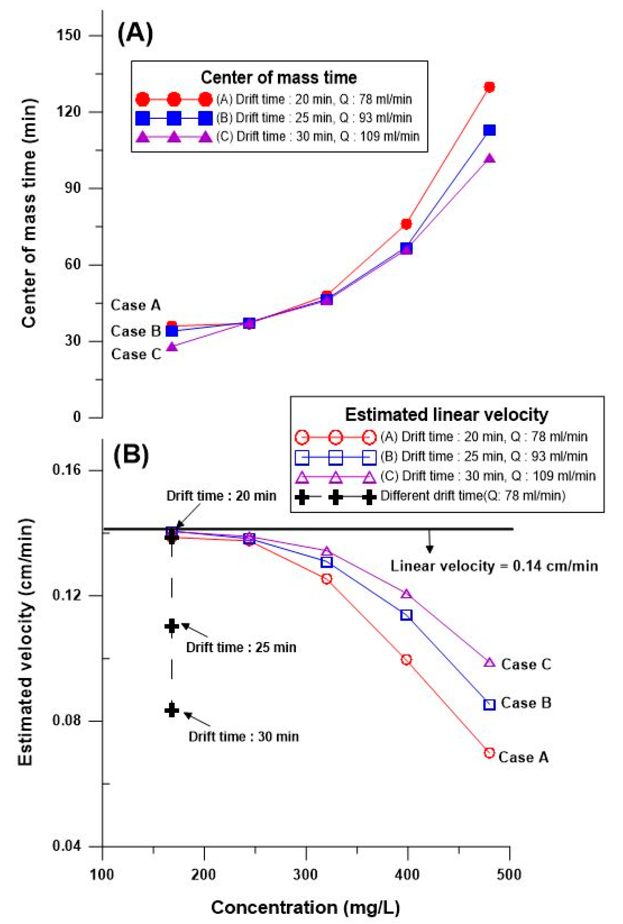
To investigate the change of tcom with the increase of the input tracer concentration, several simulations were conducted with various drift times, and the results are shown in Figure 5. When the concentration of injected tracer increased, the value of tcom also increased. For tests with the no-density effect condition (168 mg/L), Figure 5b shows decreasing linear velocity estimates with the increase of drift time (20 min → 25 min → 30 min) at the fixed pumping rate 78 mL/min. To make the initial linear velocity equal to 0.14 cm/min over the three drift times, different extraction rates were applied to the simulations (78 mL/min for 20 min of drift time, 93 mL/min for 25 min, and 109 mL/min for 30 min). The longer drift time induced the higher degree of dispersion, which makes it hard for the tracer plume to fully recover toward the extraction well, and finally, tcom increases. Regarding the increase of the tracer injection concentrations for all three cases (cases A, B, and C), a decreasing trend of the estimated linear velocity was observed (Figure 5b) because the tcom became longer for the higher injected tracer concentration (Figure 5a). Usually, we could assume that the longer tcom would make the velocity greater due to the further travel distance of the injected tracer. However, Figure 5b showed that the estimated linear velocity decreased when the tcom was increased. This can be explained by Equation (2). When the linear velocity is estimated using Equation (2), the ttotal (tcom + drift time) in the denominator is squared and the increasing rate of the denominator is greater than the numerator. In Equation (2), the travel distance of the tracer during the test can be calculated as . When the tcom increased during drift time because of density-induced sinking, the ttotal also increased and the VH can be underestimated under the travel distance of the no-density effect condition. This can cause an underestimation of the linear velocity despite the increase of tcom. In this way, the increase of tcom is not necessarily associated with the increase of linear velocity.
The horizontal travel distance of the tracer can be calculated by Hall’s equation (Equation (2)). However, when the density-induced sinking effect governs the migration pathway of the tracer with high concentration, transport directions would not be horizontal but diagonal [29,30]. This can cause a longer travel distance and lengthened tcom. However, the density-induced sinking effect can cause a shorter horizontal travel distance than that of the no-density effect condition. To confirm the difference of horizontal distance between the density-effect condition and the no-density effect condition, the horizontal travel distance was calculated using two linear velocities in Equation (4), which were obtained from (1) laboratory experiment (exact V) and (2) push-pull tests (push-pull V). The horizontal travel distance can be derived as:
where, V is the linear velocity (m/s) and tcom is the time of the center of mass at each input concentration condition(s).
In Figure 6, the horizontal distance values for estimating the linear velocity were compared with the real traveled horizontal distance values. Specifically, to draw the linear velocity (exact V) value (0.14 cm/min) at the concentration of 398 mg/L, the horizontal travel distance should be calculated as 10.6 cm for 76 min (tcom of 398 mg/L tracer injection concentration condition) under 20 min of drift time. However, the real traveled horizontal distance can be calculated as 0.10 cm/min (push-pull V estimated from Equation (2) under the density-effect condition of 398 mg/L) × 76 min (tcom of the 398 mg/L condition) and the result is 7.6 cm. The results indicate that the real horizontal travel distance for the density-induced sinking effect condition using the push-pull V can be shorter than that using the exact V. This suggests that the more reliable horizontal position information of the tracer or contaminant from the injected or contaminated well after drift time can be obtained only when the density-induced sinking effect is adjusted.
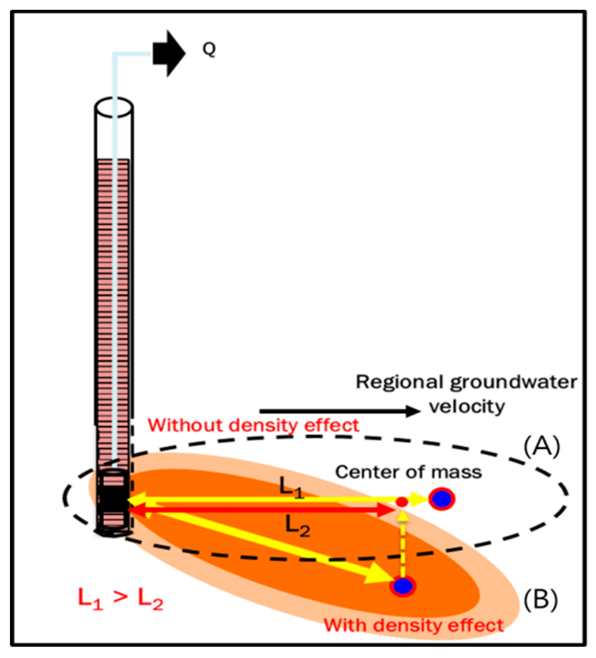
A conceptual model for estimating horizontal travel distance was made to understand the comparison between the no-density case and the density-induced sinking case (Figure 7). If the tracer plume travels horizontally along with the groundwater flow direction without the density-induced sinking effect, it can provide a good estimation of the horizontal position from the well (A). However, the density-induced sinking can affect the travel route of a dense plume as the plume sinks during transportation (B). In other words, in case B, the horizontal travel distance of a tracer plume in porous media is shorter than case A (L1 > L2).
3.3. Estimating Pumping Rate (Q) Under Various Background Velocities
The results of the laboratory tests and numerical simulations indicated that misinterpretation of the linear velocity of the groundwater was plausible when there were tracer density effects or longer drift times with a higher hydraulic gradient. In other words, interpretation of the push-pull test can be significantly affected by the various test designs. Therefore, the establishment of an appropriate pumping rate is important to estimate the exact linear velocity, which can fully cover the various transport phases of the tracer plume derived from multiple factors.
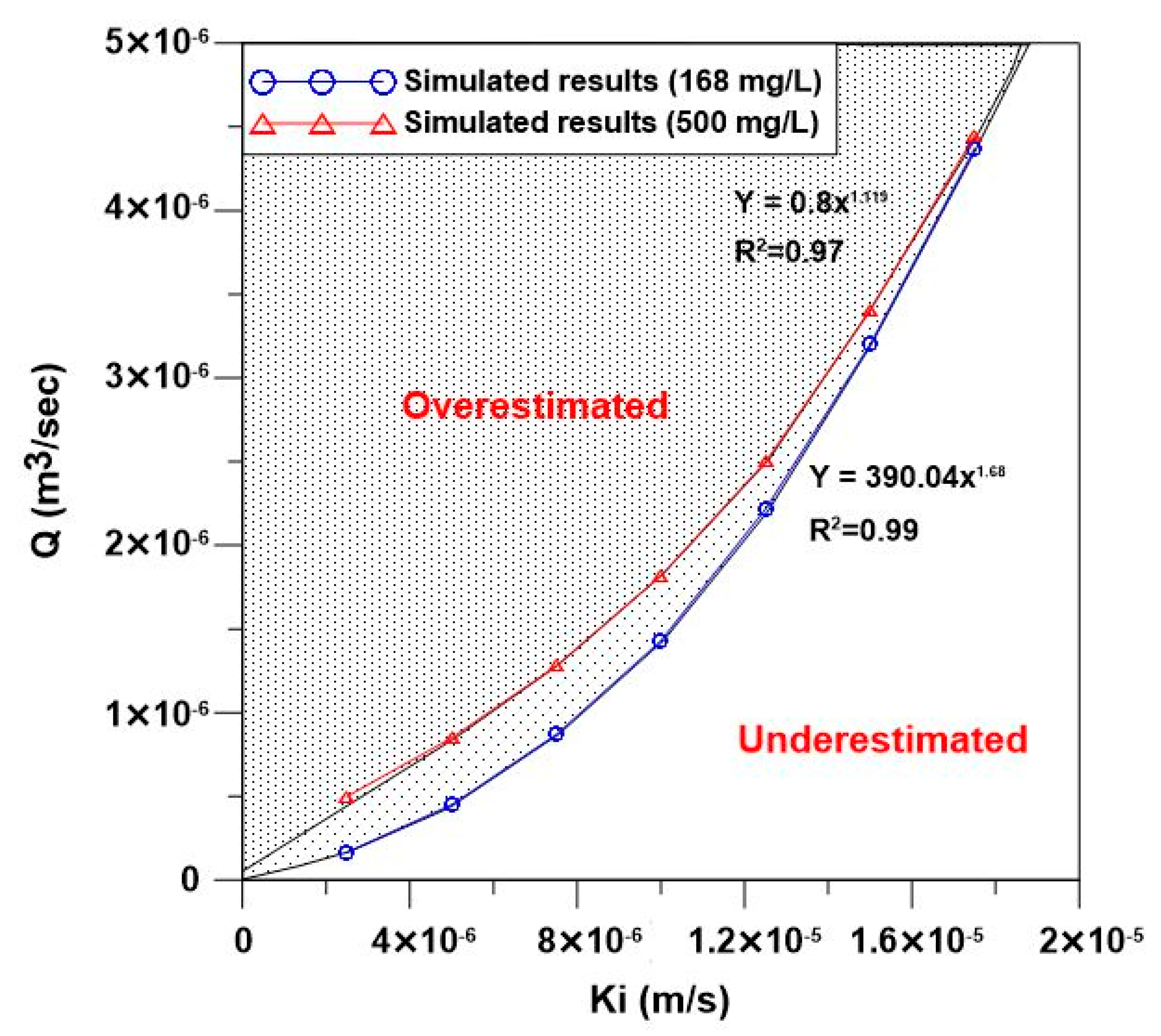
Because background groundwater flow rates vary according to sites or test conditions, various flow conditions were simulated to investigate the effect of pumping rate at each condition. The applied hydraulic gradients were increased from to in simulations, and proper pumping rates at each background flow condition are plotted in Figure 8. There are reasonable pumping rate increases as the background groundwater velocity increases. In addition, 500 mg/L of the tracer concentration condition was applied to investigate the reasonable pumping rate with the density effect. In this case, a higher pumping rate was required in the case of denser plume than the no-density effect condition. As mentioned above, the density effect caused underestimation of the linear velocity and the results supported that a higher pumping rate was required under the density-effect condition. Therefore, when there is a density-induced sinking effect, the pumping rate should be increased to obtain a more reliable linear velocity value and the difference of reasonable pumping rate between the no-density case (168 mg/L) and density-effect case (500 mg/L) became larger with the increase of the background groundwater velocity.
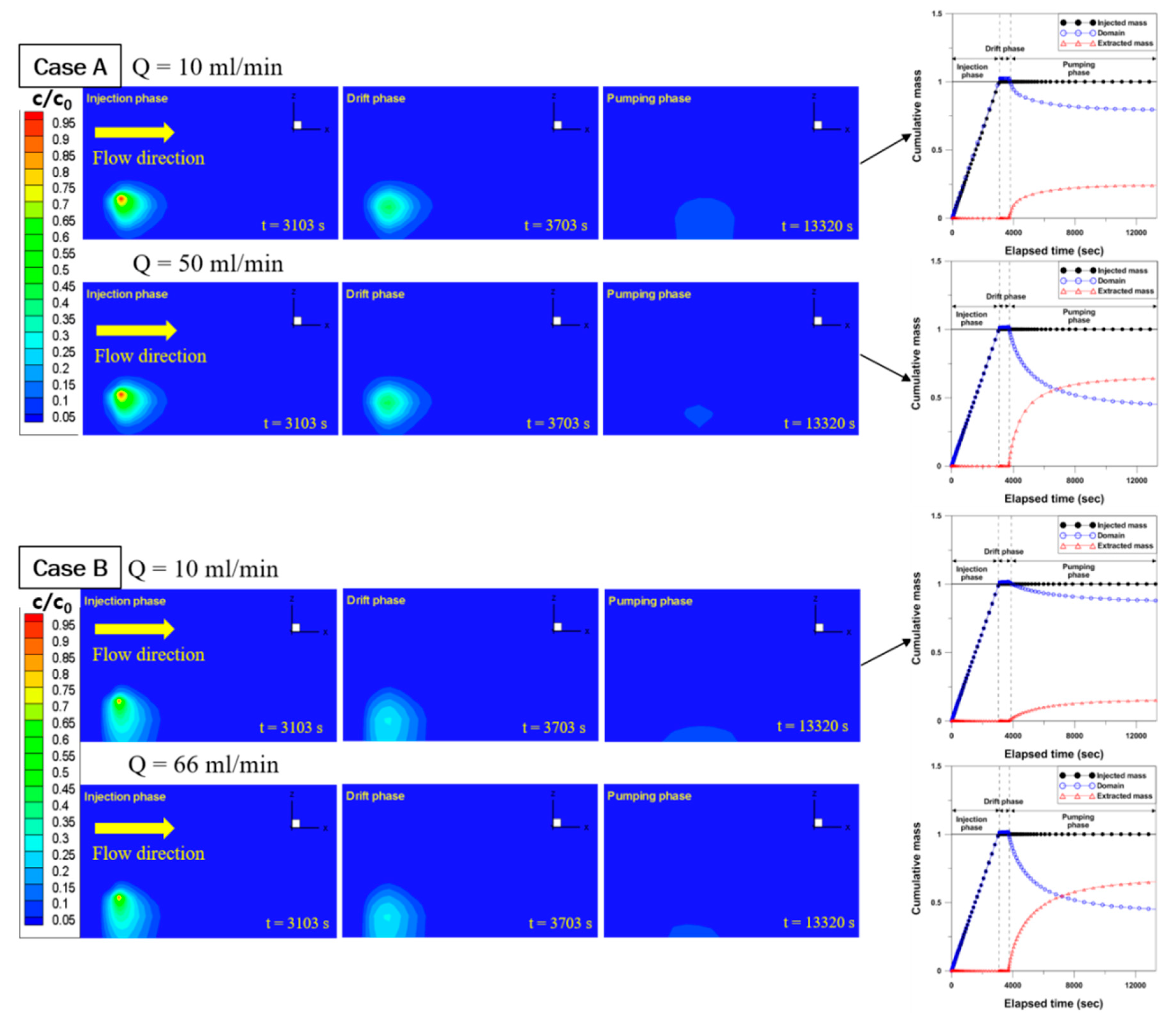
The simulated results are shown in Figure 9a (160 mg/L) and Figure 9b (500 mg/L). In the cases of applying a low pumping rate (10 mL/min) the same as the experiments, both cases showed a lot of residual (80%–85% of injected mass) in the flow field and underestimated linear velocity values were obtained due to the low pumping rate. However, in the case of applying a reasonable pumping rate (50 mL/min in the case of 160 mg/L and 66 mL/min in the case of 500 mg/L) obtained from Figure 8, both cases showed much less residual (36%–40% of injected mass) in the flow field and exact linear velocity values were obtained. Furthermore, density-induced sinking affected the tracer mass recovery rate. About 12% of the injected tracer mass was recovered under the density-effect condition, while 20% of the injected tracer mass was recovered without the density-effect condition for the pumping rate of 10 mL/min. Consequently, the higher pumping rate should be applied under the density effect to obtain a reliable linear velocity. To confirm the reliability of simulated capture zones, the results are compared with the theoretical capture zone [31] in Figure S4.
To confirm the difference of estimated linear velocity under pumping rates higher and lower than the reasonable pumping rate (Q) suggested by Figure 8, two cases of simulations were performed with 0.8 times the pumping rate (0.8 Q) and 1.2 times the pumping rate (1.2 Q). Figure S5 shows that the higher pumping rate (1.2 Q) causes overestimated linear velocity, and the lower pumping rate (0.8 Q) causes underestimated linear velocity than that by using the reasonable pumping rate (Q). Over- and under-estimation of the linear velocity according to different magnitudes of the pumping rate could be explained by the conceptual model shown in Figure 10. When the applied pumping rate is low, only part of the total injected plume could be recovered because of the small capture zone and the position of the center of mass is miscalculated as it is located near the pumping well. The incorrectly calculated center of mass can lead to the linear velocity being underestimated. In contrast to the low pumping rate, the high pumping rate can enhance the plume recovery and increase the size of the capture zone. Because pumping rate is the most sensitive parameter in Equation (2), finding a reasonable pumping rate is necessary to obtain a reliable linear velocity through the push-pull tracer test.
4. Summary and Conclusions
Laboratory-scale push-pull tracer tests were performed to investigate the factors that affect the results of push-pull tests. Although it is known that many factors affect the result of a push-pull tracer test, density effect and pumping rate have rarely been considered as important influential factors in estimating linear groundwater velocity. The influence of density and pumping rate on the estimation of the linear velocity was analyzed through laboratory-scale experiments and numerical simulations in this study.
Numerical simulations after model validation based on the experimental results showed that the condition of no-density-induced sinking is necessary to obtain the exact linear velocity estimate. As the input tracer concentration was increased, the linear velocity had a trend of underestimation because solute travel distance and direction during drift time were dependent on tracer concentration. Reasonable pumping rate should be applied during the pull phase of the test for accurate estimation of the velocity. When a high pumping rate was applied, the linear velocity had a trend of overestimation, and the low pumping rate caused underestimation of linear velocity because it produced an incorrect center of mass time (tcom). The appropriate pumping rate should be adopted to the background groundwater velocity and the higher pumping rate should be applied as the background groundwater velocity increases. Reasonable pumping rates versus background groundwater velocity for specific tracer concentrations were presented in this study.
An optimal push-pull tracer test design under various hydrogeological conditions may exist, but it is beyond the scope of this paper. In order to suggest generally applicable guidelines, it is necessary to propose approximate guidelines through additional modeling and laboratory experiments, and verify the validity by applying them in the field.
Supplementary Materials
The following are available online at https://www.mdpi.com/2073-4441/11/8/1558/s1, Figure S1: Comparison Water content (%) measured for 5 days by 5TE sensor, Figure S2: Schematic diagram of push-pull test, Figure S3: Comparison of the C/C0 value obtained from the numerical simulation (in full line) with that from the experiments (in dot) with 3 density conditions: (A) 168 mg/L, (B) 398 mg/L, (C) 1050 mg/L, Figure S4: The comparison between the theoretical capture zone and estimated capture zone by numerical simulations (R2 = 0.87), Figure S5: The comparison of estimated velocity and Darcy velocity as applying the higher (1.2 Q) and lower (0.8 Q) pumping rate.
Author Contributions
H.-H.K.: Methodology, experiment, analysis, and writing; E.-H.K.: analysis and review; S.-S.L.: analysis and review; K.-K.L.: Conceptualization, funding acquisition, and review. All authors participated in discussions and editing.
Funding
This research was funded by the “R&D Project on Environmental Management of Geologic CO2 Storage” from the KEITI (Project Number: 2018001810002). This research was also supported by the National Research Foundation of Korea (NRF) grant funded by the Ministry of Science and ICT (MSIT) of South Korean government (No. 2017R1A2B3002119).
Conflicts of Interest
The authors declare no conflict of interest.
References
- Istok, J.D.; Humphrey, M.D.; Schroth, M.H.; Hyman, M.R.; O’Reilly, K.T. Single-well, “push-pull” test for in situ determination of microbial activities. Ground Water 1997, 35, 619–631. [Google Scholar] [CrossRef]
- Lai, K.C.; Lo, I.M.; Kjeldsen, P. Natural gradient tracer test for a permeable reactive barrier in Denmark. I: Field study of tracer movement. J. Hazard. Toxic. Radioact. Waste 2006, 10, 231–244. [Google Scholar] [CrossRef]
- Qi, J.; Xu, M.; Cen, X.; Wang, L.; Zhang, Q. Characterization of Karst Conduit Network Using Long-Distance Tracer Test in Lijiang, Southwestern China. Water 2018, 10, 949. [Google Scholar] [CrossRef]
- Ptak, T.; Schmid, G. Dual-tracer transport experiments in a physically and chemically heterogeneous porous aquifer: Effective transport parameters and spatial variability. J. Hydrol. 1996, 183, 117–138. [Google Scholar] [CrossRef]
- Kass, W.; Behrens, H. Tracing Technique in Geohydrology; CRC Press/Balkema: Boca Raton, FL, USA, 1998. [Google Scholar]
- Ptak, T.; Piepenbrink, M.; Martac, E. Tracer tests for the investigation of heterogeneous porous media and stochastic modelling of flow and transport—A review of some recent developments. J. Hydrol. 2004, 294, 122–163. [Google Scholar] [CrossRef]
- Bashar, K.; Tellam, J.H. Non-reactive solute movement through saturated laboratory samples of undisturbed stratified sandstone. Geol. Soc. Lond. Spec. Publ. 2006, 263, 233–251. [Google Scholar] [CrossRef]
- Gouze, P.; Le Borgne, T.; Leprovost, R.; Loads, G.; Poidras, T.; Pezard, P. Non-Fickian dispersion in porous media: 1. Multiscale measurements using single-well injection withdrawal tracer tests. Water Resour. Res. 2008, 44. [Google Scholar] [CrossRef] [Green Version]
- Huang, J.; Christ, J.A.; Goltz, M.N. Analytical solutions for efficient interpretation of single-well push-pull tracer tests. Water Resour. Res. 2010, 46. [Google Scholar] [CrossRef]
- Istok, J.D. Push-Pull Tests for Site Characterization; Springer Science and Business Media: Berlin/Heidelberg, Germany, 2012. [Google Scholar]
- Hansen, S.K.; Berkowitz, B.; Vesselinov, V.V.; O’Malley, D.; Karra, S. Push-pull tracer tests: Their information content and use for characterizing non-Fickian, mobile-immobile behavior. Water Resour. Res. 2016, 52, 9565–9585. [Google Scholar] [CrossRef]
- Paradis, C.J.; McKay, L.D.; Perfect, E.; Istok, J.D.; Hazen, T.C. Push-pull tests for estimating effective porosity: Expanded analytical solution and in situ application. Hydrogeol. J. 2018, 26, 381–393. [Google Scholar] [CrossRef]
- Meigs, L.C.; Beauheim, R.L. Tracer tests in a fractured dolomite: 1. Experimental design and observed tracer recoveries. Water Resour. Res. 2001, 37, 1113–1128. [Google Scholar] [CrossRef] [Green Version]
- Leap, D.I.; Kaplan, P.G. A single-well tracing method for estimating regional advective velocity in a confined aquifer: Theory and preliminary laboratory verification. Water Resour. Res. 1988, 24, 993–998. [Google Scholar] [CrossRef]
- Hall, S.H.; Luttrell, S.P.; Cronin, W.E. A method for estimating effective porosity and ground-water velocity. Ground Water 1991, 29, 171–174. [Google Scholar] [CrossRef]
- Hwang, H.T. Experimental and Numerical Sensitivity Analyses on Push-Drift-Pull Tracer Tests. Master’s Thesis, Seoul National University, Seoul, Korea, 2004. [Google Scholar]
- Hebig, K.H.; Zeilfelder, S.; Ito, N.; Machida, I.; Marui, A.; Scheytt, T.J. Study of the effects of the chaser in push-pull tracer tests by using temporal moment analysis. Geothermics 2015, 54, 43–53. [Google Scholar] [CrossRef]
- Wang, Q.; Zhan, H.; Wang, Y. Single-well push-pull test in transient Forchheimer flow field. J. Hydrol. 2017, 549, 125–132. [Google Scholar] [CrossRef]
- Simmons, C.T.; Fenstemaker, T.R.; Sharp, J.M. Variable-density groundwater flow and solute transport in heterogeneous porous media: Approaches, resolutions and future challenges. J. Contam. Hydrol. 2001, 52, 245–275. [Google Scholar] [CrossRef]
- List, E.J. The Stability and Mixing of a Density-Stratified Horizontal Flow in a Saturated Porous Medium. Ph.D. Thesis, California Institute of Technology, Pasadena, CA, USA, 1965. [Google Scholar]
- Schincariol, R.A.; Schwartz, F.W. An experimental investigation of variable density flow and mixing in homogeneous and heterogeneous media. Water Resour. Res. 1990, 26, 2317–2329. [Google Scholar] [CrossRef]
- Oostrom, M.; Dane, J.H.; Güven, O.; Hayworth, J.S. Experimental investigation of dense solute plumes in an unconfined aquifer model. Water Resour. Res. 1992, 28, 2315–2326. [Google Scholar] [CrossRef]
- Oostrom, M.; Hayworth, J.S.; Dane, J.H.; Güven, O. Behavior of dense aqueous phase leachate plumes in homogeneous porous media. Water Resour. Res. 1992, 28, 2123–2134. [Google Scholar] [CrossRef]
- Zhang, H.; Schwartz, F.W.; Wood, W.W.; Garabedian, S.P.; LeBlanc, D.R. Simulation of variable-density flow and transport of reactive and nonreactive solutes during a tracer test at Cape Cod, Massachusetts. Water Resour. Res. 1998, 34, 67–82. [Google Scholar] [CrossRef]
- Barth, G.R.; Illangasekare, T.H.; Hill, M.C.; Rajaram, H. A new tracer-density criterion for heterogeneous porous media. Water Resour. Res. 2001, 37, 21–31. [Google Scholar] [CrossRef] [Green Version]
- Abramoff, M.D.; Magelhaes, P.J.; Ram, S.J. Image processing with ImageJ. Biophotonics Int. 2004, 11, 36–42. [Google Scholar]
- Therrien, R.; McLaren, R.G.; Sudicky, E.A.; Panday, S.M. Hydrogeosphere: A Three-Dimensional Numerical Model Describing Fully-Integrated Subsurface and Surface Flow and Solute Transport; Groundwater Simulations Group, University of Waterloo: Waterloo, ON, Canada, 2010. [Google Scholar]
- Shackelford, C.D.; Daniel, D.E. Diffusion in saturated soil. I: Background. J. Geotech. Geoenviron. 1991, 117, 467–484. [Google Scholar] [CrossRef]
- Istok, J.D.; Humphrey, M.D. Laboratory investigation of buoyancy-induced flow (plume sinking) during two-well tracer tests. Ground Water 1995, 33, 597–604. [Google Scholar] [CrossRef]
- Beinhorn, M.; Dietrich, P.; Kolditz, O. 3-D numerical evaluation of density effects on tracer tests. J. Contam. Hydrol. 2005, 81, 89–105. [Google Scholar] [CrossRef]
- Grubb, S. Analytical model for estimation of steady-state capture zones of pumping wells in confined and unconfined aquifers. Ground Water 1993, 31, 27–32. [Google Scholar] [CrossRef]
Figure 1.
Schematic experimental setup for the laboratory-scale push-drift-pull tracer test.

Figure 2.
(A) Model domain and (B) boundary condition for the numerical simulation.

Figure 3.
Breakthrough curves under different tracer input density obtained from laboratory-scale push-drift-pull tracer tests (case (A): 10 min of drift time, 3.0 × 10⁻³ hydraulic gradient, case (B): 5 min of drift time, 1.2 × 10⁻² hydraulic gradient).
Figure 3.
Breakthrough curves under different tracer input density obtained from laboratory-scale push-drift-pull tracer tests (case (A): 10 min of drift time, 3.0 × 10⁻³ hydraulic gradient, case (B): 5 min of drift time, 1.2 × 10⁻² hydraulic gradient).

Figure 4.
The results of laboratory tests to visualize the movement of tracer with different concentrations ((A): The position of tracer plume after 30 min, (B): Center position of tracer plumes every 5 min analyzed by ImageJ).
Figure 4.
The results of laboratory tests to visualize the movement of tracer with different concentrations ((A): The position of tracer plume after 30 min, (B): Center position of tracer plumes every 5 min analyzed by ImageJ).

Figure 5.
Center of mass time (tcom) and estimated linear velocity from the varied input tracer concentration (Br) for fifteen cases (case A: 20 min of drift time, case B: 25 min of drift time, case C: 30 min of drift time).
Figure 5.
Center of mass time (tcom) and estimated linear velocity from the varied input tracer concentration (Br) for fifteen cases (case A: 20 min of drift time, case B: 25 min of drift time, case C: 30 min of drift time).

Figure 6.
A comparison of the horizontal distance values needed in estimating Darcy velocity with the real horizontal distance values in various drift time and density conditions.
Figure 6.
A comparison of the horizontal distance values needed in estimating Darcy velocity with the real horizontal distance values in various drift time and density conditions.

Figure 7.
The conceptual model of the migration of tracer plume under the no-density effect condition and the density-effect condition (L1: horizontal distance of no-density case, L2: horizontal distance of density case).
Figure 7.
The conceptual model of the migration of tracer plume under the no-density effect condition and the density-effect condition (L1: horizontal distance of no-density case, L2: horizontal distance of density case).

Figure 8.
The obtained reasonable pumping rates under various background groundwater velocity conditions for two concentration cases: 168 mg/L (triangles) and 500 mg/L (circles).
Figure 8.
The obtained reasonable pumping rates under various background groundwater velocity conditions for two concentration cases: 168 mg/L (triangles) and 500 mg/L (circles).

Figure 9.
Numerical simulation results in the no-density effect condition (case (A), 160 mg/L) and the density-effect condition (case (B), 500 mg/L) at three time points (t = 3103 s: the end of the injection phase, t = 3703 s: the end of the drift phase, and t = 13,320 s: the end of the pumping phase) with different pumping rates.

Figure 10.
The conceptual model of the effect of pumping rate on estimating linear velocity applying the low pumping rate (left) and the high pumping rate (right).
Figure 10.
The conceptual model of the effect of pumping rate on estimating linear velocity applying the low pumping rate (left) and the high pumping rate (right).


Table 1.
Measured hydraulic properties of sand.
| Parameter | Porous Medium (Sand) |
|---|---|
| Particle size (mm) | 1.28 |
| Bulk density (g/cm3) | 1.65 |
| Effective porosity | 0.32 |
| Field capacity | 0.02 |
| Hydraulic conductivity (cm/min) | 15 ± 0.93 |
Table 2.
Tracer test conditions for various concentrations.
| Test | Hydraulic Gradient | Initial Br Concentration (mg/L) | Test Volume (mL) | Injection Rate (mL/min) | Pumping Rate (mL/min) | Drift Time (min) |
|---|---|---|---|---|---|---|
| 1 | 0.003 | 168 | 300 | 6 | 10 | 10 |
| 2 | 0.003 | 398 | 300 | 6 | 10 | 10 |
| 3 | 0.003 | 1050 | 300 | 6 | 10 | 10 |
| 4 | 0.003 | 2450 | 300 | 6 | 10 | 10 |
| 5 | 0.012 | 168 | 300 | 6 | 10 | 5 |
| 6 | 0.012 | 2050 | 300 | 6 | 10 | 5 |
| 7 | 0.012 | 2450 | 300 | 6 | 10 | 5 |
Table 3.
Input parameters for the numerical simulation.
| Parameter | Value |
|---|---|
| Aquifer properties | |
| Aquifer K | 2.5 × 10⁻³ m/s |
| Porosity | 0.34 |
| Specific storage | 2.3 × 10⁻⁴ m−1 |
| Longitudinal dispersivity | 0.03 m |
| Transverse dispersivity | 0.015 m |
| Vertical transverse dispersivity | 0.015 m |
| Fluid properties | |
| Fluid density | 998.23 kg/m3 |
| Fluid viscosity | 1.00 × 10⁻³ kg m−1s−1 |
| KBr diffusion coefficient | 2.02 × 10⁻⁹ m2/s |
© 2019 by the authors. Licensee MDPI, Basel, Switzerland. This article is an open access article distributed under the terms and conditions of the Creative Commons Attribution (CC BY) license (http://creativecommons.org/licenses/by/4.0/).
Share and Cite
MDPI and ACS Style
Kim, H.-H.; Koh, E.-H.; Lee, S.-S.; Lee, K.-K. Biased Estimation of Groundwater Velocity from a Push-Pull Tracer Test Due to Plume Density and Pumping Rate. Water 2019, 11, 1558. https://doi.org/10.3390/w11081558
AMA Style
Kim H-H, Koh E-H, Lee S-S, Lee K-K. Biased Estimation of Groundwater Velocity from a Push-Pull Tracer Test Due to Plume Density and Pumping Rate. Water. 2019; 11(8):1558. https://doi.org/10.3390/w11081558
Chicago/Turabian StyleKim, Hong-Hyun, Eun-Hee Koh, Seong-Sun Lee, and Kang-Kun Lee. 2019. "Biased Estimation of Groundwater Velocity from a Push-Pull Tracer Test Due to Plume Density and Pumping Rate" Water 11, no. 8: 1558. https://doi.org/10.3390/w11081558
Note that from the first issue of 2016, this journal uses article numbers instead of page numbers. See further details here.