Modelling of Sediment Exchange between Suspended-Load and Bed Material in the Middle and Lower Yellow River, China

1
Key Laboratory of Yellow River Sediment Research, Yellow River Institute of Hydraulic Research, Yellow River Conservancy Commission, Zhengzhou 450003, China
2
Key Laboratory of Water Cycle and Related Land Surface Processes, Institute of Geographic Sciences and Natural Resources Research, Chinese Academy of Sciences, Beijing 100101, China
3
University of Chinese Academy of Sciences, Beijing 100049, China
*
Authors to whom correspondence should be addressed.
Water 2019, 11(8), 1543; https://doi.org/10.3390/w11081543
Submission received: 26 June 2019
/
Revised: 17 July 2019
/
Accepted: 22 July 2019
/
Published: 25 July 2019
(This article belongs to the Section Hydrology)
Abstract
:The focus of this paper is on studying novel approaches to estimate sediment exchange between suspended-load and bed material in an unsteady sediment-laden flow with fine-grained sand. The erosion-deposition characteristics of the channel have close relation with the variation of size compositions of both suspended-load and bed material. These aims are addressed by deducing the sediment exchange equations from the mass conservation perspective and establishing a river-sediment mathematical model based on the theory. The model is applied in the middle and lower Yellow River, China, and calibrated and verified under both deposition and erosion conditions using a generalized channel and a large quantity of measured data in the Yellow River basin. The results indicate that the grading curves of suspended-load and bed material calculated by the mathematical model are close to those of the measured data. The temporal and spatial variations in the mean sizes of suspended-load and bed material, flow rate, sediment concentration and erosion or deposition volume estimates during the entire flood process can be accurately predicted. The model performance is considered acceptable for determining the sediment exchange process and the change in channel morphology for unsteady sediment-laden flow.
1. Introduction
Rivers are important sources of water on the earth which are continuously changing, and sediment exchange is one of the most powerful agents in the river environment [1,2]. Sediment exchange transfigures the river morphology by long-term degradation and aggradation of channel beds via erosion and deposition. Sediments in a natural river, including suspended-load, bed-load, and bed material, are usually non-uniform and their size compositions strongly influence the flow capacity and consequent riverbed evolution [3,4,5]. In most alluvial rivers with fine-grained sand in plains (e.g., the middle and lower Yellow River), the proportion of bed-load is low and the sediment exchange between suspended-load and bed material dominates channel morphology change [6,7]. The variations in size compositions of suspended-load and bed material are closely related to erosion-deposition characteristics of the channel [8,9]. The erosion-deposition process is rather complex, which is affected by the interactions between turbulence structures and initiation of particles movement [10]. During an erosion or deposition process, particle coarsening or fining may occur in the same reach simultaneously, which results in the size gradation change of suspended-load and bed material even in the quasi-equilibrium condition, i.e., the amounts of erosion and deposition in the reach can balance each other [11]. Such processes can have a direct effect on the evolution of river forms during flooding. A change in the morphology of a river can threaten channel stability, which can create local scours around hydraulic installations [12]. Evaluating sediment exchange between suspended-load and bed material, therefore, is critical for the long-term prediction of channel morphology change for alluvial rivers with fine-grained sand [13,14,15].
Sediment exchange in alluvial rivers has gained much attention by researchers for years and has been extensively studied using various approaches [16,17]. Among other research methods, laboratorial experimenting is traditional and effective [18]. Jr and Mehta [19] carried out an experiment in a counter-rotating annular flume to explore the exchange between suspended sediment and cohesive bed material. Wang et al. [20] studied the relationship between the bed shear stress and suspended sediment concentration in an annular flume. Zanden et al. [17] presented novel insights into suspended sediment concentrations and fluxes under a large-scale laboratory breaker bar. Qin et al. [14], Yossef and Vriend [21] explored various mechanisms of sediment exchange between the main channel and the groyne fields in a mobile-bed laboratory flume.
Many statistical models for sediment exchange were developed in recent years. Aalto et al. [22] investigated the processes of sediment exchange and channel migration rates along the Strickland River through sampling and Geographic Information System (GIS) analysis. Sinnakaudan et al. [23] focused on sediment transport in high gradient rivers and developed a total-load formula by using the multiple linear regression model [24]. Tayfur et al. [25] and Pektaş [26] used principal component analysis and cluster analysis to identify some significant non-dimensional parameters of sediment transport. Moreover, machine learning based models such as neural networks, fuzzy logic, and support vector machines, were also developed to estimate sediment exchange in recent studies [27,28]. All those machine learning models have a black box nature with limited information inside the models, therefore, they can hardly be expressed as explicit formulas.
Undoubtedly, numerical studies have significantly advanced the understanding of sediment exchange processes and the ability to predict sediment transport rates in alluvial rivers [29]. There has been a plethora of such mathematical models over the last few decades. Many 1D models were developed to simulate the size variations of bed sediment [30,31,32], suspended-load [33], and the hyper-concentration flow [34,35] in alluvial channels. Rudorff et al. [36] predicted the variation in channel-floodplain suspended sediment exchange along a 140 km reach of the lower Amazon River for two decades (1995–2014) with a 2D hydraulic model. Jing et al. [29] proposed a 2D depth averaged Renormalization Group (RNG) k–ε sediment model to simulate the long- and short-term sediment transport and bed deformation in rivers with continuous bends. Aziaian et al. [37], Qamar and Baig [38] applied the CCHE2D model to simulate the non-uniform sediment transport and channel migration in unsteady flows. Yang et al. [39] refined a 2D depth-integrated numerical model based on the Depth Integrated Velocity and Solute Transport (DIVAST) model to simulate bed evolution in the Yellow River Delta, China, from 1992 to 1995. Li and Duffy [40] put forward a 2D high-order model by fully coupling equations of shallow water flow, non-equilibrium sediment transport, and morphological bed evolution in rivers and floodplains. Recently, several 3D models were also developed to simulate sediment movement. Delft3D is capable of modelling 3D hydrodynamics and sediment transport using a finite difference method [11]. Van Rijn et al. [41] took advantage of DELFT3D to simulate the bed evolution of an artificial sand ridge near Hoek van Holland, located close to the harbor of Rotterdam in the Netherlands. Chung and Eppel [42] examining the sensitivity of sediment transport and bed morphology to the variations of bed slopes, grain sizes, and the non-hydrostatic pressure term based on a 3D hydrodynamic and sediment transport model. Franz et al. [43] developed a comprehensive 3D morphological model to predict suspended sediment transport and bed evolution for the Tagus Estuary, Portugal, based on the local hydrodynamic conditions.
To simulate the sediment exchange, most of the above numerical models divide sediment particles into several size groups, treat each group with various methods, and assign some exchanging rules between groups [44]. For instance, Jha and Bombardelli [45] addressed the transport of multi-disperse suspended sediment mixtures in open channels, via the use of the two-fluid model. They confirmed the volumetric concentration of the sediment corresponding to several particle size classes. Bui and Rutschmann [46] developed a sediment transport module for fractional sediment transport using a multiple layer model with the size-fraction method that takes into account the influence of size distribution of the grains on bed-surface on the flow field and bed evolution. Caliskan and Fuhrman [47] coupled a 1D vertical turbulence-closure flow model with sediment transport capabilities to incorporate graded sediment mixtures by treating the bed and suspended load individually for each grain fraction. Franz et al. [43] utilized a morphological model to estimate the non-uniform sediment exchange in natural systems composed of multiple sediment classes. Considering the interactive influences between particles of different sizes have not been well understood, these types of numerical models are always confronted with more complicated computational difficulties and bring considerable numerical inaccuracy [45].
This paper aims to gain new insights into the principles of sediment exchange during riverbed evolution of the alluvial rivers with fine-grained sand, and proposes a novel river-sediment mathematical model to calculate the grain size, composition and exchange of both suspended-load and bed material with no need to divide the sediment into groups based on particle force analysis and mass conservation. The model is applied in the context of the middle and lower Yellow River, China. Although the annual runoff of the Yellow River basin is only approximately 2% of China’s total, it directly supports 12% of the national population and feeds 15% of the irrigation area [48]. Catastrophic floods and droughts appeared frequently in the Yellow River basin over thousands of years in Chinese history, so a large quantity of flow measurements and sediment samples have been collected along the river and stored in a database. This database provides a useful means for validating the model performance. In addition, in the middle and lower Yellow River, bed-load is rare, and the sediment exchange between suspended-load and bed material dominates changes in bed morphology [6,7]. Given its global importance as a large river, the Yellow River is an important case example to evaluate the strengths and potential weaknesses of the theoretical approach for sediment exchange between suspended-load and bed material in alluvial rivers with fine-grained sand presented in this paper.
In this paper, we first present a theoretical framework and establish a river-sediment mathematical model for unsteady flow. Then, a generalized channel is set up to qualitatively analyze and calibrate the model for both deposition and erosion conditions. Finally, the proposed model is applied in the eroded and silted river reaches of the middle and lower Yellow River to investigate its performance. Good agreement between the numerically simulated results and the field measurements is obtained, indicating that the newly-developed model is capable of predicting the sediment gradation and exchange in the middle and lower Yellow River with reasonable accuracy.
2. Study Site and Data
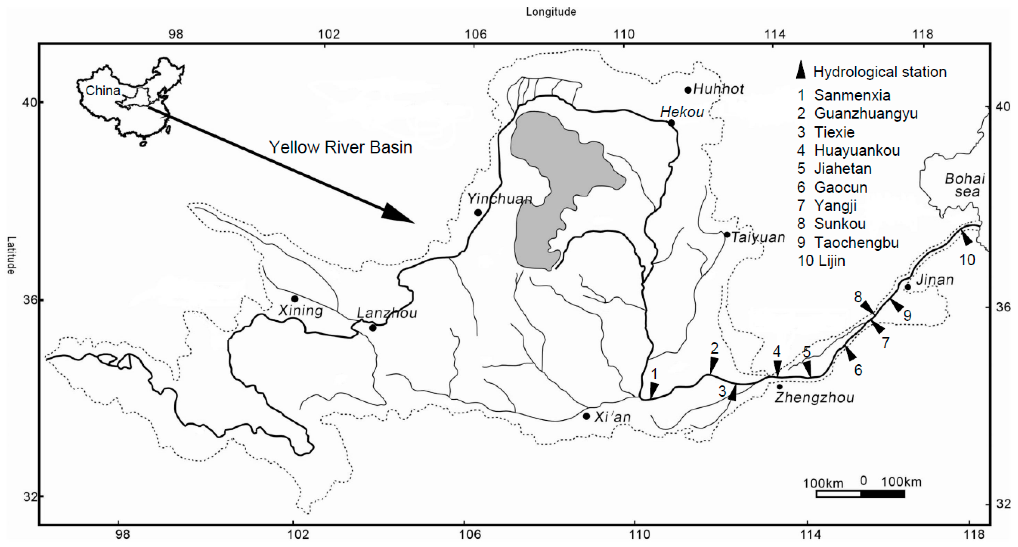
The Yellow River, also called the Huanghe in Chinese, is the second longest river in China. This river is located between 96–119° E longitude and 32–42° N latitude, with a drainage area of c. 753,000 km2 and a mean stem length of 5464 km (Figure 1). The river originates from the world’s largest plateau (the Tibetan Plateau), wanders through northern semiarid regions, crosses the loess plateau, passes through the eastern plain, and finally discharges into the world’s largest ocean (the Pacific Ocean) [49]. As seen in Figure 1, the Yellow River basin is usually divided by its physical characteristics into three water source areas: the upper (above Hekou), middle (between Hekou and Huayuankou) and lower (below Huayuankou) reaches [50].
The Yellow River is noted for its relatively low water discharge compared with its very high sediment load: the river has a mean annual water discharge of only approximately 0.7% of the Amazon (the largest river in the world) and 4.5% of the Yangtze (the largest river in China) but an annual sediment load almost equal to that of the Amazon and more than twice that of the Yangtze [51]. The sediment load from the Yellow River basin is estimated to contribute approximately 6% of the total global river load to the oceans [50]. Due to its high sediment concentration and rapid sedimentation rate, the average sediment deposition in the lower reach was 1.58 × 10⁸ t/a (t represents unit ton and a represents age) from 1950 to 2004 [52].
This study focuses on the middle and lower Yellow River as a typical alluvial reach with fine-grained sand (Figure 1). The flow and sediment data collected at 10 hydrological stations along the reach, e.g., Sanmenxia, Tiexie, Huayuankou, Jiahetan, Sunkou, and Lijin, were obtained from the Yellow River Conservancy Commission (YRCC). The physical characteristics of the middle and lower reaches in the Yellow River basin are presented in Table 1.
To investigate the applicability of the theoretical approach of sediment exchange and the river-sediment mathematical model presented in this paper, the modelling calculation was conducted using the data of the flood season from the middle and lower Yellow River in 1977 and 1999 to 2002 [48].
Notably, 1977 was a typical year of high sediment load. At Sanmenxia station, the annual water volume was only 30.7 billion m3, and the annual sediment load was 2.08 billion t. In July 1977, the maximum flow was 8100 m3/s, the maximum measured sediment concentration was 535 kg/m3, and the composition of the suspended-load was coarse at Huayuankou station. The hyper-concentrated flood in the lower Yellow River caused channel erosion and beach deposition. Because the deposition volume of beach areas was far greater than the erosion volume of the main channel, the entire channel experienced substantial sediment deposition. During the process of sediment deposition along the channel, the composition of the suspended-load became increasingly fine grained.
After the flood season in 1999, the river reach from Tiexie to Lijin exhibited bed material gradation at 31 measurement sections. The initial composition of the bed material in the lower section was determined according to the distance between sections using an interpolation method. Based on the measured data over three years, the entire channel of the middle and lower Yellow River experienced erosion. Before the flood season in 2002, bed material gradation was observed in the partial middle and lower Yellow River, and the composition of bed material exhibited obvious coarsening compared with that in 1999.
3. Methodology
3.1. Mathematical Model
Based on force analyses of sediment particles under turbulent flow conditions, the variations in gradation of suspended sediment and bed material are derived, as seen in Appendix A1 in detail. According to the principle of mass conservation, unsteady formulas of suspended sediment and bed material exchange are established for the alluvial rivers, as seen in Appendix A2 in detail. The variations of the key parameter, i.e., the mean size of the entrained particles (dc), the average settling velocity of non-uniform sediment in muddy water (ωs) and other factors describing the erosion and deposition processes are investigated as seen in Appendix A3. According to these theories, we establish both 1D and 2D river-sediment mathematical models for unsteady flow in this paper. The basic equations of the models are as follows.
1D river-sediment mathematical model:
2D river-sediment mathematical model:
where subscripts “i” and “j” represent each cross section and sub-cross section, respectively, m is the number of sub-cross sections, Zw is the water level, K is the discharge modulus, α1 and α2 are the momentum correction coefficients of flow and lateral inflow, respectively, α* is the distribution coefficient of sediment concentration in an equilibrium state, Zb is the average bed elevation of each cross section, C is Chezy coefficient, S* is the vertical averaged sediment carrying capacity of the flow, and dcp and Dcp are the mean sizes of total suspended sediment and bed material, respectively. Full details of the other definitions of the model are presented in the Appendix A. The primary parameters during the sediment exchange process in above models can be ascertained as follows.
where , which is the average settling velocity of non-uniform sediment in clear water; , which is the mean size of bed material load when channel morphology change reaches dynamic equilibrium; , which is the maximum particle diameter under critical conditions for sediment suspension; is the particle diameter of relatively coarse bed material; and M is a coefficient.
3.2. Modelling Procedure and Scenario Setting
When solving the mathematical models, the uncoupled solution is adopted. Firstly, solve the continuity and dynamic equations of flow and obtain the hydraulic elements. Then, solve the continuity equation of sediment and riverbed deformation equation, and ascertain the erosion and deposition process of the riverbed. Finally, calculate dcp and Dcp. The solving process proceeds alternately and circularly till the simulation period is over.
Two simulation stages are designed in this study. The first stage is to calibrate the presented models. In the second stage, abundant simulations of a hyper-concentrated flood of the lower Yellow River are conducted to evaluate the applicability of the mathematical models of sediment exchange for both the deposition and erosion conditions.
3.3. Model Calibration and Verification
To preliminarily calibrate the model presented in this paper, we carry out qualitative analysis and calculation of a generalized channel. According to the on-site sediment composition and river bed gradient in the middle and lower Yellow River [48], the generalized channel is set as 100 km long and 200 m wide with a vertical gradient of 1. The initial mean and median sizes of the bed material (Dcp and D50) are set at 0.125 mm and 0.1 mm, respectively. The roughness coefficient of the riverbed is set at 0.012. The steady flow rate is set at 530 m3/s, and the initial water depth is 2 m. For the deposition conditions, the sediment concentration S of the inlet is set at 100 kg/m3, and the mean and median sizes of the suspended-load (dcp and d50) are set at 0.04 mm and 0.032 mm, respectively. For the erosion conditions, the sediment concentration S of the inlet is set at 1 kg/m3, and the mean and median sizes of the suspended-load (dcp and d50) are set at 0.015 mm and 0.012 mm, respectively. The temporal and spatial variations in the mean and median sizes of suspended-load and bed material of the generalized channel are obtained by the model simulation.
Moreover, we have derived sediment gradation equations in light of force analyses of sediment particles (Appendix A1). The sediment gradation can be calculated based on the simulation results to verify the mathematical models. The sediment gradation equations are as follows:
where is the normal distribution function.
To evaluate the performance of the newly developed model, the calculated and measured values are compared using the Nash-Sutcliffe efficiency coefficient (NSE) and Pearson correlation coefficient r defined as follows:
where Xm and Xc are the measured and calculated values, respectively. NSE and r are commonly used to quantitatively assess the predictive power of hydrological models [53,54]. If NSE > 0.5 and r > 0.6, the model performance is considered to be acceptable.
3.4. Model Settings and Parameters
To investigate the applicability of the theoretical approach of sediment exchange and the river-sediment mathematical model presented in this paper, measured data from a hyper-concentrated flood of the lower Yellow River in July 1977 were used in the analysis for the deposition conditions, and the river reach used for verification extended from Huayuankou to Jiahetan (Figure 1). The initial bed material gradation in each section was determined according to the measured gradation data from Huayuankou to Jiahetan before the flood season based on the interpolation method. The outlet boundary condition was controlled by the stage-discharge relationship of Jiahetan station in 1977.
The temporally variable values of the inlet flow and sediment concentration in the model were determined according to the measured data from Huayuankou station using a temporal interpolation method. Because the quantity of measured gradation data for the suspended-load was small, the modeled results differ from the actual results if the temporal interpolation method is directly applied. As a result, a relation involving dcp, Q and S was established through regression analysis.
The value of dcp of the suspended-load corresponding to the measurement time of the sediment concentration was obtained using Equation (10), and the existing measured value of dcp was retained. Then, the values of dcp during the entire computational period were determined using the temporal interpolation method.
To verify the newly proposed approaches for erosion conditions in this paper, the data collected from the middle and lower Yellow River during the period between November 1999 and October 2002 were used in this analysis, and the river reach used for verification extended from Tiexie to Lijin (Figure 1). The measured water and sediment values and the composition of the suspended-load at Xiaolangdi station were set as the inlet boundary conditions. The initial topography was controlled by the measured sections of the partial middle and lower Yellow River after the flood season in 1999. The water level at the end of the model was controlled using the stage-discharge relationship observed at Lijin station in the same year.
4. Results and Discussion
4.1. Results of Model Calibration
4.1.1. Deposition Conditions
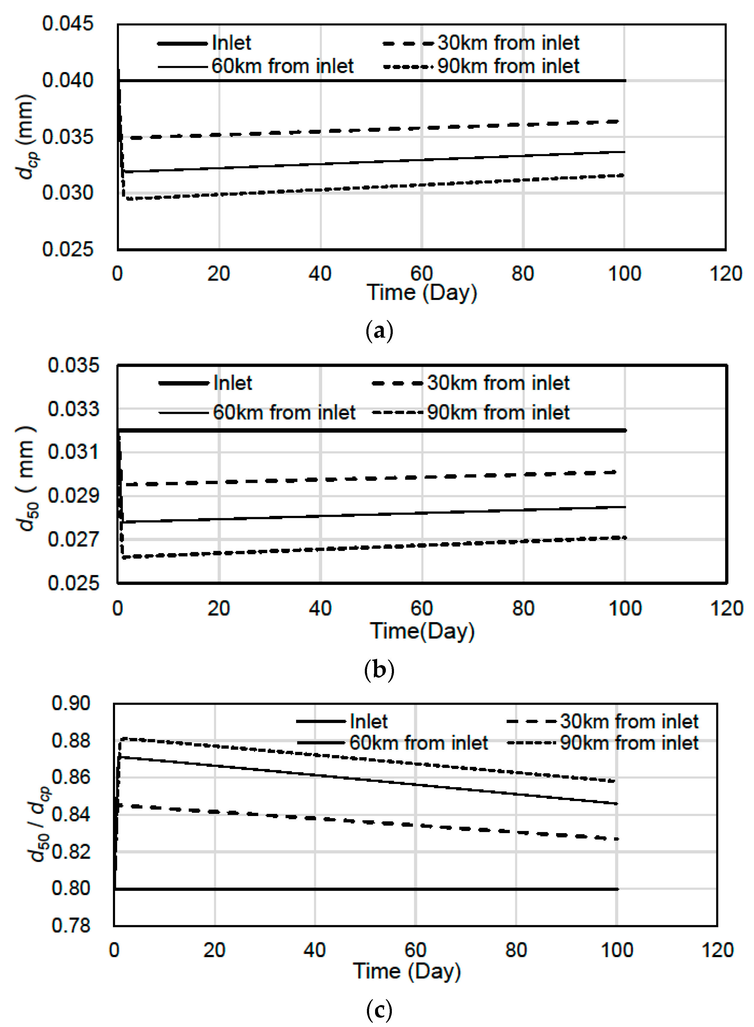
Figure 2 shows the temporal variations in , and with different cross sections along the channel. In the silting process, and decrease along the channel, and increases along the channel. The degree of sediment fining of the upper reach (30–60 km) is larger than that of the lower reach (60–90 km) over an equal distance and time frame. During the calculated period, the sediment-carrying capacity of the flow gradually increases with the increase in the vertical gradient as a result of deposition, so the fining effect of the suspended-load has a tendency to decrease.
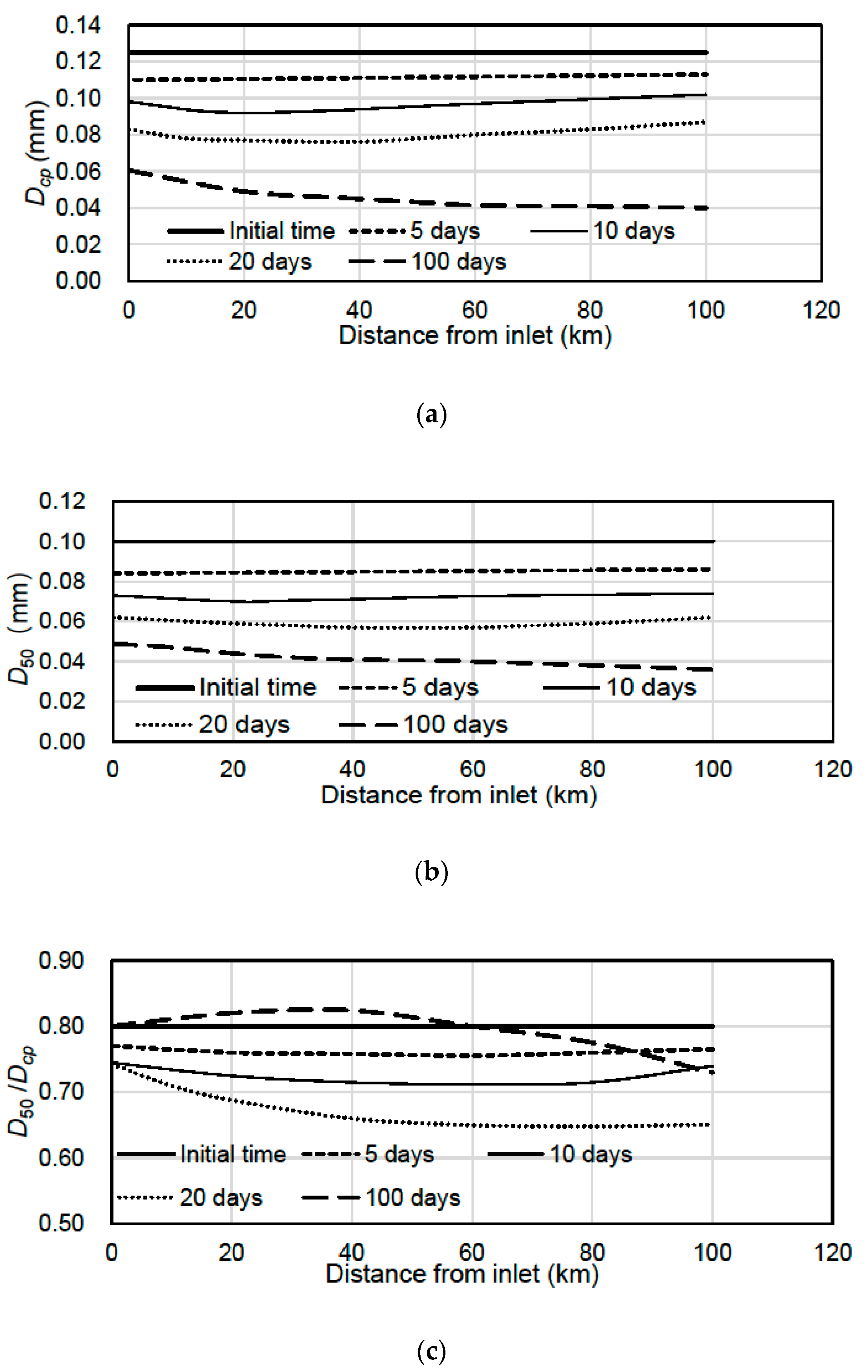
Figure 3 presents the spatial variations in , and along the channel with different deposition times. As shown, the composition of bed material gradually becomes finer in the silting process. The fining process starts from the upper reach to the lower reach. In the early stage, the bed material becomes more non-uniform as abundant suspended-load silts on the bed ( decreases in the same cross section). With increasing deposition, the bed material gradation becomes relatively uniform ( increases with a calculation time of 100 days).
4.1.2. Erosion Conditions
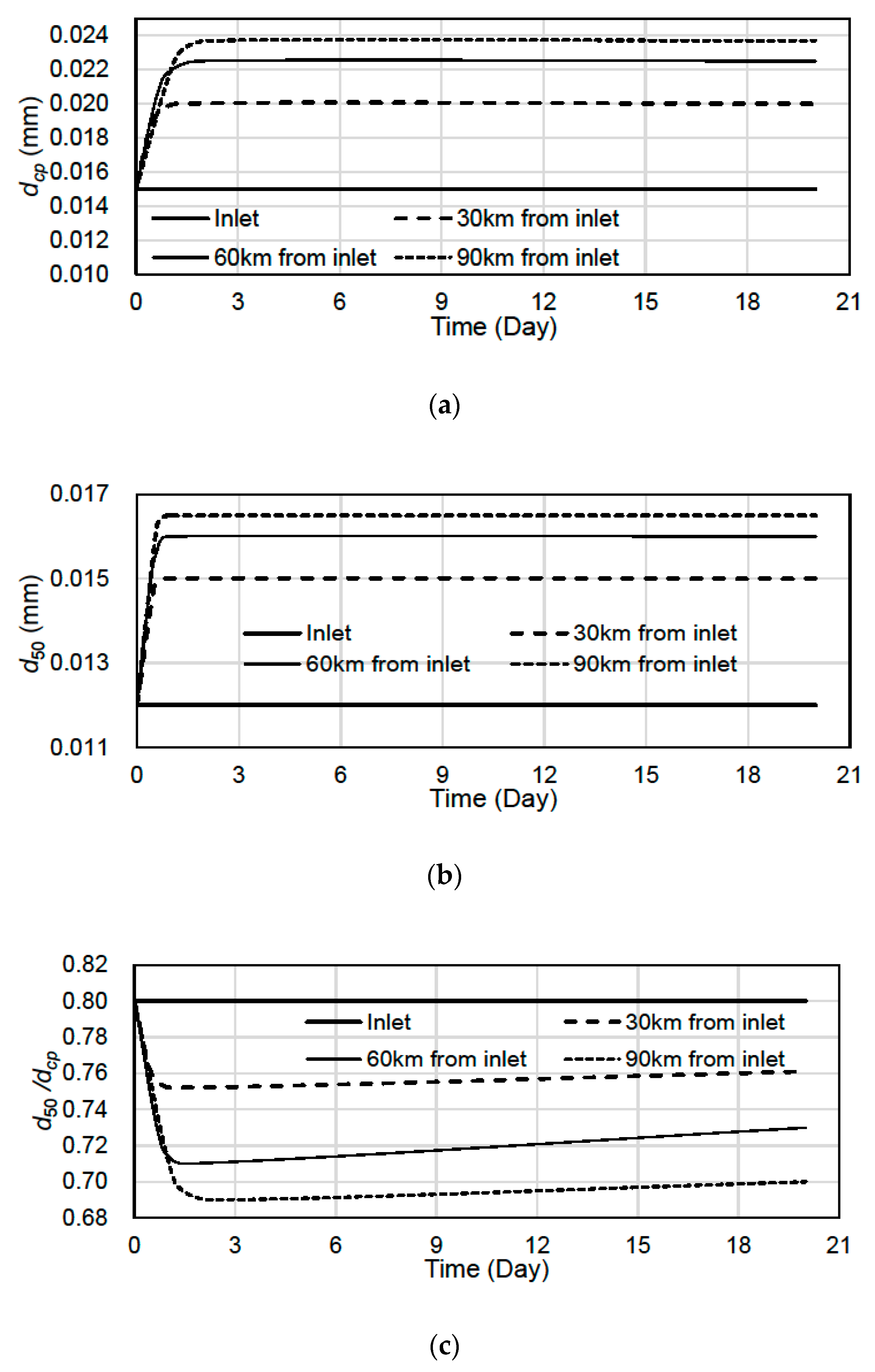
As shown in Figure 4, and increase along the channel during scouring, and decreases along the channel, which means the composition of the suspended-load becomes increasingly non-uniform. The degree of sediment coarsening of the upper reach is larger than that of the lower reach over the same time. The sediment-carrying capacity of flow gradually decreases with the decreasing vertical gradient of the riverbed during the erosion process, and the coarsening effect of the suspended-load tends to decrease.
As shown in Figure 5, bed scouring starts from the upper reach to the lower reach with the increase in and during scouring, and the coarsening effect on the bed material in the upper reach is larger than that in the lower reach. In the early stage of erosion, the bed material becomes increasingly non-uniform as the finer bed material is scoured up to the flow, so decreases in the same cross section. With the development of erosion, more and more fine particles are washed away, so the bed material gradation gradually becomes uniform. As the erosion quantity of the upper reach is larger than that of the lower reach, in some sections of the upper reach begins to increase with the calculation time of 10 days.
In light of the calculation results of the generalized channel under deposition or erosion conditions, the variation in sediment gradation and exchange is consistent with the basic rules of sediment movement. Thus, the model presented in this paper is considered to be preliminarily reliable.
4.2. Application and Verification
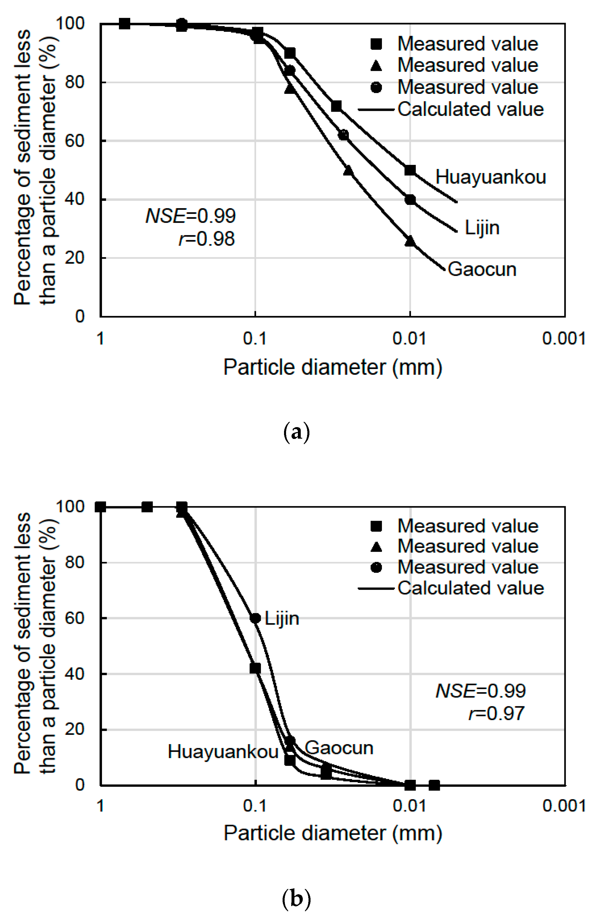
4.2.1. Verification of the Sediment Gradation Calculation
We calculated the sediment gradation based on the model and Equations (6) and (7). Figure 6a,b compare the calculated grading curves of the suspended-load and bed material, respectively, with the measurements at three hydrological stations in the lower Yellow River, i.e., Huangyuankou, Lijin, and Gaocun stations. The model can clearly be applied to calculate the suspended-load and bed material gradation of a natural river with a wide range of particle diameters.
4.2.2. Verification of the Sediment Exchange Calculation for Deposition Conditions
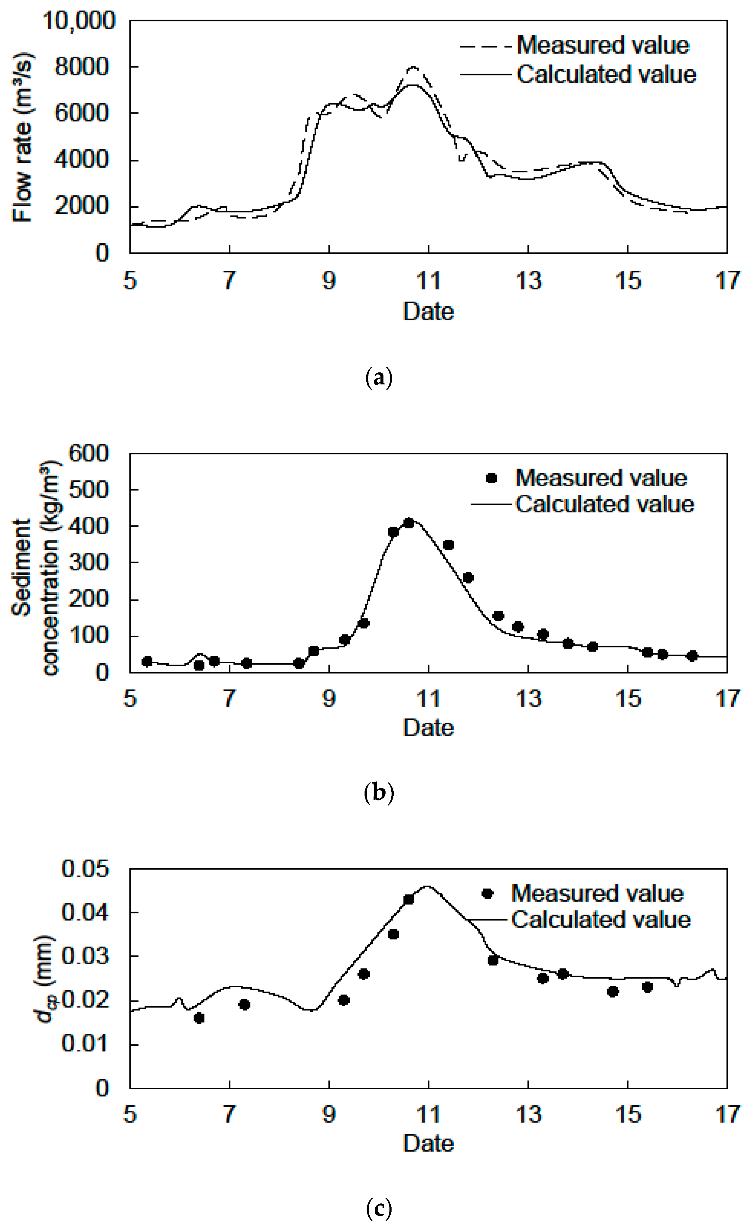
Based on the model simulation results, Figure 7 shows the comparative results of the calculated and measured values of the flow rate (NSE = 0.95 and r = 0.95), sediment concentration (NSE = 0.98 and r = 0.98), and dcp (NSE = 0.89 and r = 0.97). The results of the exchange simulation method of the suspended-load and bed material presented in this paper exhibit good agreement with the measured data for the peak flow, flood transmission time, maximum sediment concentration and its emergence time. The results present the high calculation accuracy of the flow and sediment concentration during the entire process compared to the results of traditional methods. Moreover, the values of and variations in dcp for the suspended-load are relatively close to the measured values and trends. The established mathematical model can further improve the accuracy and functionality of the simulated evolution of hyper-concentrated floods and variations in riverbed deposition in the lower Yellow River. Thus, the method of simulating exchange processes involving suspended-load and bed material presented in this paper is applicable for deposition conditions in natural rivers.
4.2.3. Verification of the Sediment Exchange Calculation for Erosion Conditions
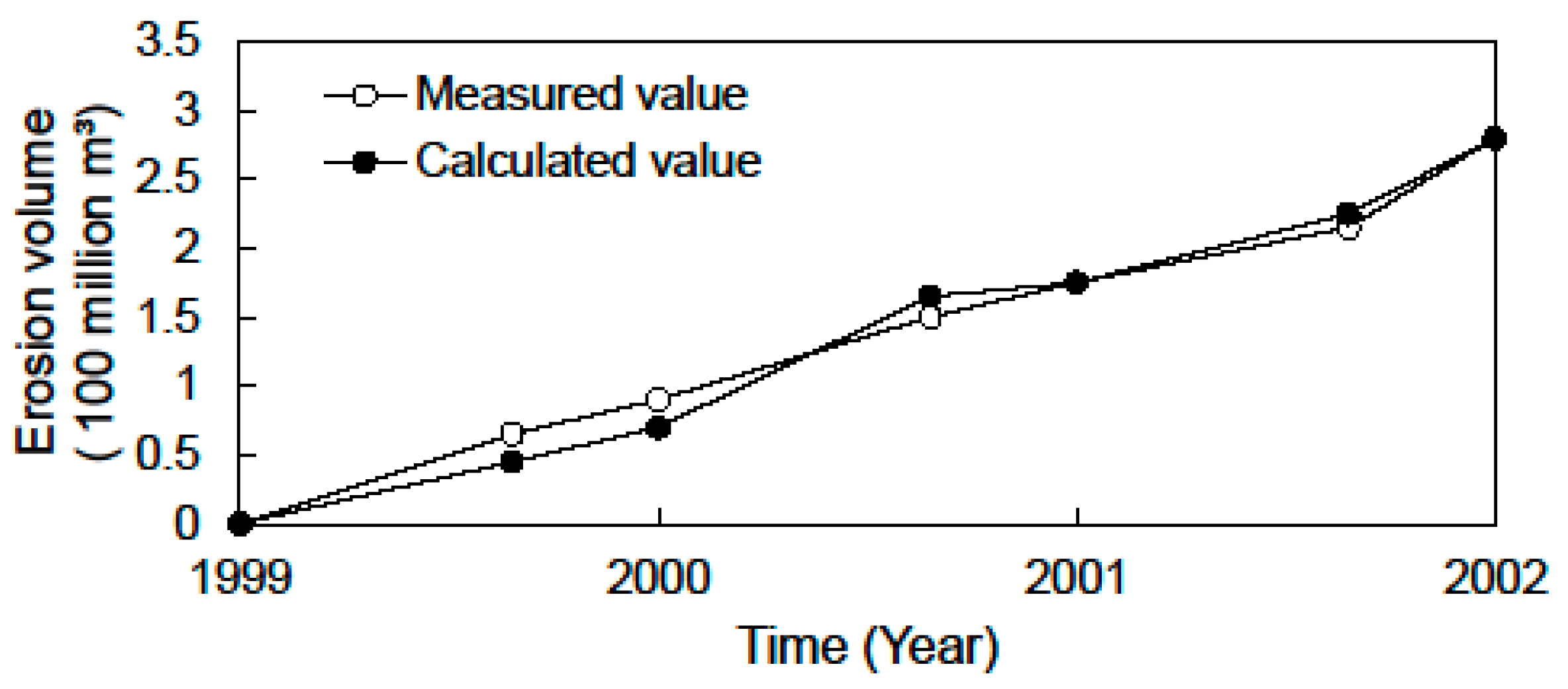
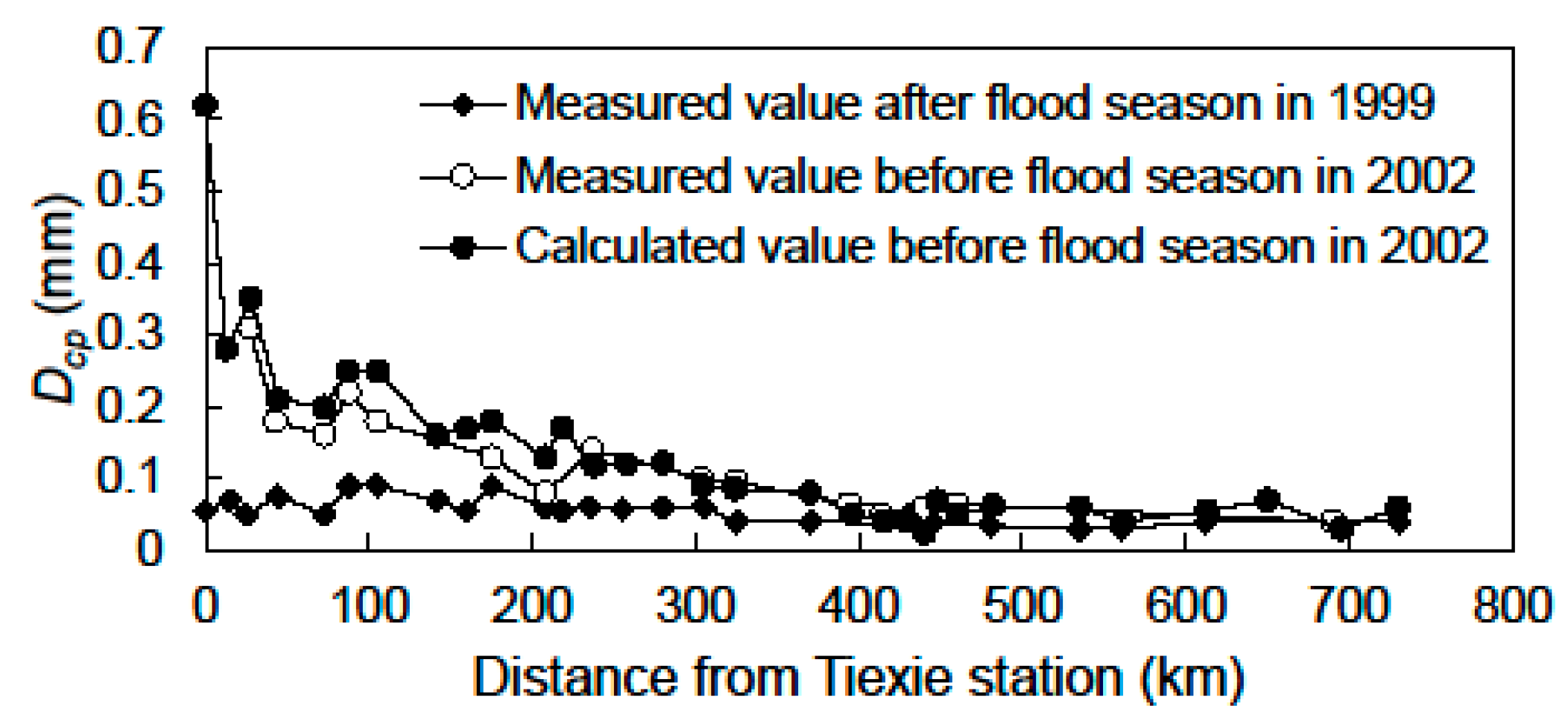
Figure 8 displays the comparative results of the calculated and measured erosion processes for the entire lower channel (NSE = 0.98 and r = 0.98). Figure 9 displays the comparative results of the mean size of the bed material Dcp for the major channel surface of the middle and lower Yellow River before the flood season in 2002 (NSE = 0.78 and r = 0.93). According to the comparative results, the evolution process and distribution of erosion in the middle and lower Yellow River calculated by the model agree well with the measured data. Additionally, the coarsening of bed material by erosion and exchange between bed material and suspended-load are supported by the results. The computational accuracy of the model satisfies the production requirement. As a result, the method of simulating the exchange process of suspended-load and bed material presented in this paper is applicable under erosion conditions in natural rivers.
5. Conclusions
In this paper, we have systematically presented a novel approach for simulating the gradation and exchange of suspended sediment and bed material for the alluvial rivers with fine-grained sand. Based on force analyses of sediment particles under turbulent flow conditions, the variations in sediment gradation are calculated. According to the principle of mass conservation, 1D, 2D and 3D unsteady formulas of suspended sediment and bed material exchange are established. This approach avoids the adverse factors compared with the calculation methods based on the fractional carrying capacity for graded sediment, and a river-sediment mathematical model is built in light of the theoretical approach. The model is applied to the case of the middle and lower Yellow River, China, which belongs to representative unsteady sediment-laden flow with high concentration of fine-grained sand. Some of the most important river-sediment features during flood events are reproduced, including the sediment particle diameter, flow rate, sediment concentration, erosion and deposition volume, etc.
The results imply that the grading curves of the suspended-load and bed material calculated are relatively close to those of the measured data. The predicted values of the mean sizes of the suspended-load and bed material match well with the associated measured values, and the computational accuracy of the flow, sediment concentration and erosion and deposition volume estimates during the entire flood process is greatly improved. In contrast with the traditional methods, the newly developed approaches could not only provide an effective tool for simulating the sediment exchange between suspended-load and bed material for sediment-laden flow, but also improve the ability of numerical models in estimating sediment concentration and channel morphology change during flood events.
Author Contributions
Conceptualization, L.Z. and E.J.; methodology, L.Z.; software, W.Z.; validation, D.C.; formal analysis, W.Z.; investigation, W.Z.; writing—original draft preparation, W.Z.; writing—review and editing, D.C. and E.J.; supervision, L.Z.; funding acquisition, L.Z.
Funding
This research was funded by National Key R&D Program of China (grant No. 2017YFC0405204), National Natural Science Foundation of China (grant No. 51539004, 51709124, 51779242, 41330751), and Young Elite Scientists Sponsorship Program by CAST (grant No. 201938).
Acknowledgments
The authors are indebted to the reviewers and editors for their valuable comments and suggestions.
Conflicts of Interest
The authors declare no conflict of interest.
Appendix A
Appendix A.1. Sediment Gradation
Appendix A.1.1. Gradation of Suspended Sediment
Considering equilibrium suspension in turbulence, the forces exerted on a suspended particle should balance each other along vertical direction:
where G is gravity, L is the turbulent uplift force, γs and γ are the unit weights of sediment and the water, respectively, is the density of water, is the uplift force coefficient, is the particle diameter, and is the velocity component along vertical direction, which influences the movement of suspended sediment when .
Substituting Equation (A2) into Equation (A1) yields the following expression
Equation (A3) expresses the minimum needed to suspend the grain with . For non-uniform suspended-load, calculated by Equation (A3) can suspend particles with diameters equal to or less than . Assume the representing size of particles (d) suspended by is proportional to :
where is a coefficient.
According to Hou [55], the value of is related to the particle size. The dimensionless form of can be written as follows:
where is the mean size of total suspended sediment, is a coefficient, and is an exponent.
Substituting Equations (A4) and (A5) into Equation (A3), the following formula can be obtained:
where and .
With the assumption of normal distribution, the probability distribution of can be written as follows.
According to Equations (A6) and (A7), the probability distribution function (PDF) of d can be deduced in the following form.
Calculating the mathematical expectation of , can be described as follows:
where Γ is the gamma function.
Reorganizing Equation (A9), the following Equation (A10) is obtained.
Substituting Equation (A10) into Equation (A8), Equation (A8) can be written as follows.
Integrating d in Equation (A11) from 0 to , the weight percentage of the suspended sediment with sediment particle diameters of less than can be expressed as follows:
where is the normal distribution function.
= 0.5 when . Equation (A12) can be simplified as follows:
where is the median diameter of the suspended sediment.
According to Equation (A13), there is one-to-one match between and . To facilitate the calculation, Equation (A13) can be approximated by the Equation (A14):
Besides, Equation (A12) can be also simplified as follows.
Appendix A.1.2. Gradation of Fine-Grained Bed Material
Bed material in the lower reach of an alluvial river with fine-grained sand is composed of fine particles with sizes in the same order as the suspended-load. The particles can follow the flow moving closely, which facilitates the exchange between suspended-load and bed material. The threshold of incipient sediment motion can be expressed as the force balance along vertical direction:
where is the eddy lift force, is the uplift force coefficient associated with incipient motion, is the particle diameter, and is the near-bed velocity along vertical direction. In the form of expression, Equations (A16) and (A17) are similar to Equations (A1) and (A2), respectively. With similar treatment, the gradation of fine-grained bed material can be expressed as follows:
where and are the median and mean sizes of bed material, respectively.
Appendix A.2. Sediment Exchange
Appendix A.2.1. 1D Equation
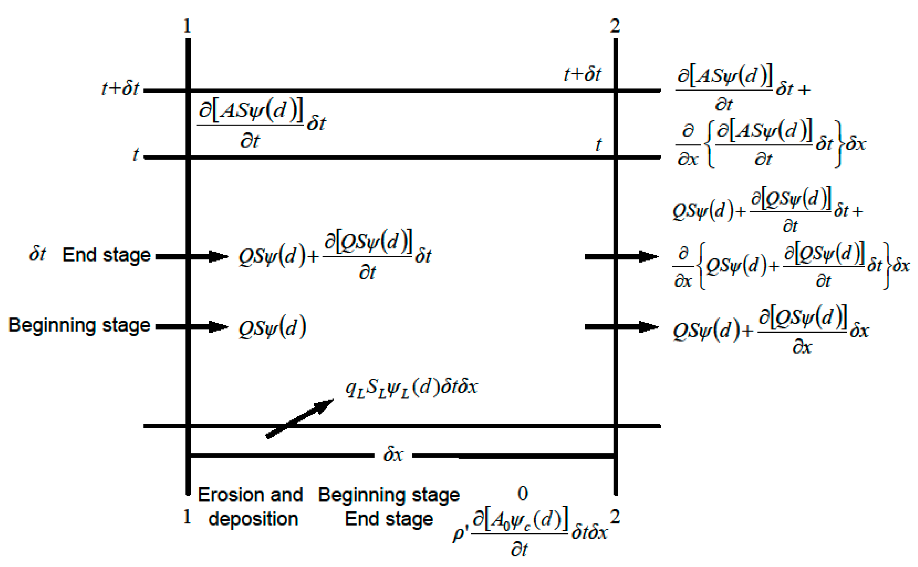
As illustrated in Figure A1, the net inflow () of sediment of size into the reach in the period of :
where is the distance between two sequent cross sections; is the discharge; is the sediment concentration; and are the cross-sectional area and its change, respectively; is time period; is the sediment dry density; and are the size distribution function for the inflow and lateral inflow, respectively; and are the discharge per unit width and concentration for lateral inflow, respectively.
Figure A1.
Schematic diagram of 1D suspended sediment and bed material exchange.

The total increase of sediment () of size within the reach in the period of :
The increase of the sediment () of size from lateral inflow and riverbed:
Following the mass conservation law:
Substituting Equations (A20)–(A22) into Equation (A23), divided by , and multiplied by before integrating over the section as . Ignoring higher-order small quantities, the variations in size of the suspended-load during sediment exchange can be expressed as follows:
where , and are the mean size of particles from bed and lateral inflow, respectively.
Let denotes the thickness of the mixed layer on bed in the period , is the PDF of bed material size, and Z is the bed elevation. The mess of bed material of size per unit width be written as follows.
In the beginning stage:
In the end stage:
Erosion and deposition:
Following the mass conservation law:
Substituting Equations (A25)–(A27) into Equation (A31), divided by , and multiplied by before integrating over the section as :
Because , Equation (A29) can be simplified to the following form.
Appendix A.2.2. Horizontal 2D Equation
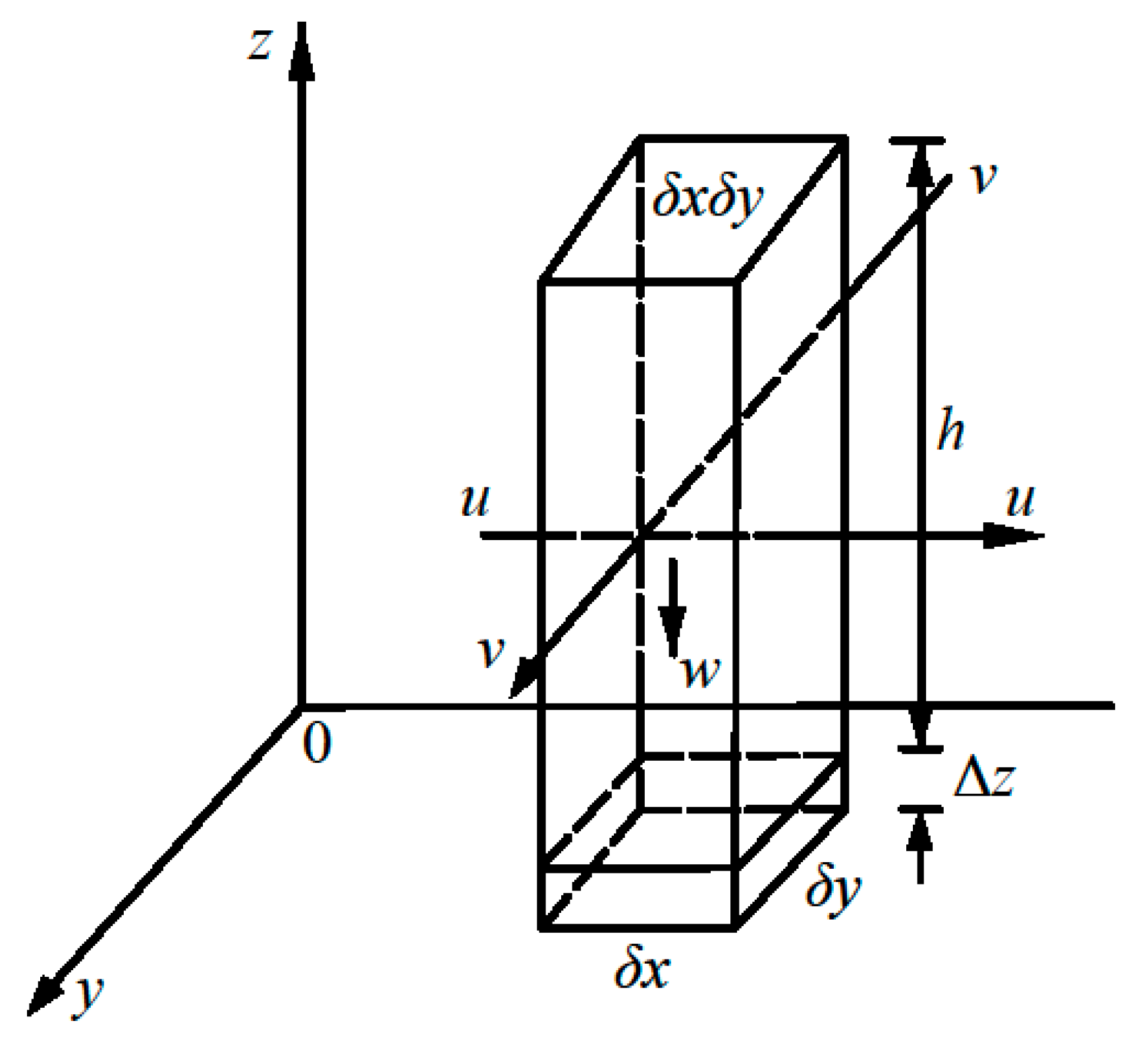
As shown in Figure A2, using the similar method for 1D equation, one can obtain the horizontal 2D equation for mean size of suspended sediment in unsteady sediment-laden flow:
where and are the diffusion coefficients of suspended sediment in the x- and y-directions, respectively; and is the bed change. It is assumed that vertical acceleration can be neglected, the flow is incompressible, and each group of sediment particles moves with the flow.
Figure A2.
Schematic diagram of horizontal 2D suspended sediment and bed material exchange. The control volume is a unit prism with bottom and the depth h. x and y are coordinates; y is the direction perpendicular to flow; u and v are the velocity components in the x- and y-directions, respectively.

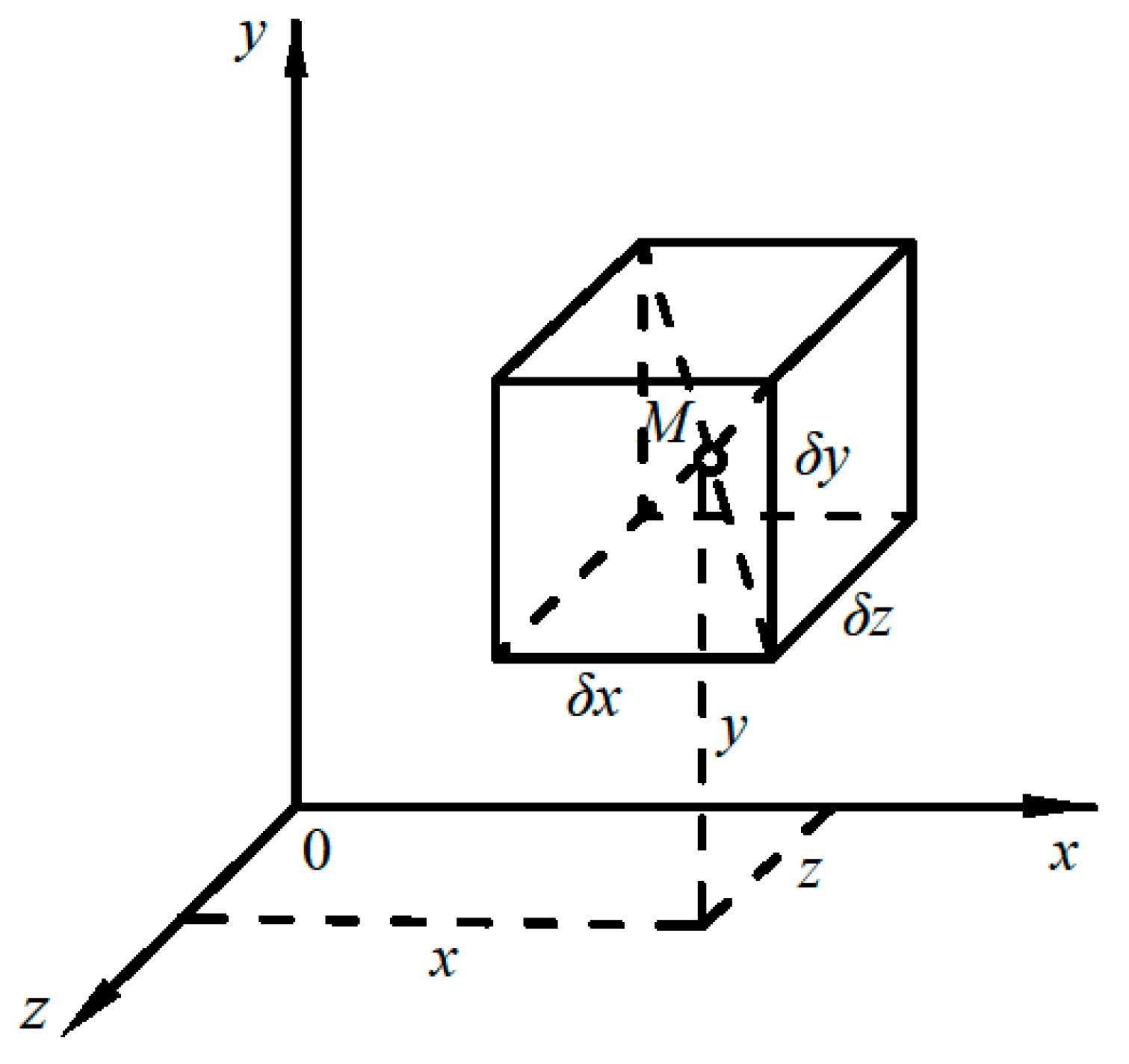
Appendix A.2.3. 3D Equation
As shown in Figure A3, similarly, 3D equation can be established based on mass conservation law. It is noted that the suspended-load of size entering the control volume in period along the y-direction is given by , where is the settling velocity of .
where S represents the time-averaged sediment concentration at M; is the average settling velocity of the non-uniform suspended mix; , and are the velocity components in the x-, y- and z-directions, respectively; , and are the diffusion coefficients of suspended sediment in the x-, y- and z-directions, respectively. It is assumed that the flow is incompressible and each group of sediment particles moves with the flow.
Figure A3.
Schematic diagram of a regular hexahedron element. The control volume is a regular hexahedron element with centroid M and coordinates ().
Figure A3.
Schematic diagram of a regular hexahedron element. The control volume is a regular hexahedron element with centroid M and coordinates ().

Appendix A.3. Key Parameters
Appendix A.3.1. The Mean Size of Entrained Particles
The coarser suspended particles settle on the riverbed in a silting process, while the finer bed material is entrained during a scouring process. The exchange of sediment continues even when the channel morphology change reaches a dynamic equilibrium, but the mass and mean size of exchanging sediment from both sides will be equal.
The mean size of entrained particles () is one of the key parameters in examining the sediment exchange. Theoretically, should be between mean size of suspended-load and mean size under critical conditions for sediment suspension . The section deduce the expression of in the process of silting and scouring, respectively.
Let denotes the mean size of bed material load when channel morphology change reaches dynamic equilibrium. In a silting process, the value of dc is between the values of and :
where m is a weight coefficient between 0 and 1 related to the degree of non-equilibrium of the reach. If the situation is far from the equilibrium, is close to , otherwise is close to .
Assume m:
where is the thickness of deposition; S and h are sediment concentration and water depth in an unit prism, respectively; α is an exponent.
The mean size of the residual particles remained in the water after deposition:
Substituting Equations (A33) and (A34) into Equation (A35) yields:
The sorting of suspended sediment during a silting process is significant when the concentration is relatively low. Since when , the relationship between α, and can be deduced by calculating the limitation of Equation (A36):
Substituting Equations (A34) and (A37) into Equation (A33), can be written as follows.
Similarly, there exists the following expression of in a scouring process:
where is a weight coefficient between 0 and 1 related to the degree of non-equilibrium of the reach. If the situation is far from the equilibrium, is close to , otherwise is close to .
Assume :
where is the bed elevation change; is the thickness of sediment exchanging layer. is an exponent.
The mean size of the residual particles remained in the water after deposition:
when the riverbed is strongly eroded, and is close to the particle diameter of relatively coarse bed material . Substituting Equation (A39) into Equation (A41) and calculating the limit of Equation (A41), can be formulated as follows.
Additionally, substituting Equations (A40) and (A42) into Equation (A39), Equation (A39) can be written as follows.
According to the research on riverbed deformation [56], the riverbed deformation formula can be expressed as follows:
where is the average settling velocity of non-uniform sediment from erosion and deposition materials, and and are the sediment concentration and the saturated sediment concentration at the river bottom, respectively. and are coefficients.
When the riverbed erodes, the erosion depth of the riverbed can be written as follows.
Because the thickness of direct-exchange layer can be considered the largest possible erosion depth of the riverbed without considering the inhibiting effect of the suspended sediment in the flow, Equation (A45) can be used to form Equation (A46):
where is the average settling velocity of .
Let and , where is the vertical average sediment concentration and is the vertical averaged sediment carrying capacity of the flow. Dividing Equation (A45) by Equation (A46) yields Equation (A47).
The coefficient in Equation (A47) is the unsaturated sediment coefficient , which can be calculated as follows [56].
The values of and in Equation (A47) can be calculated based on the following equation: [57], which is the average settling velocity of non-uniform sediment in clear water, and is the settling velocity of uniform sediment with particle diameter in clear water. Substituting , and Equation (A48) into Equation (A47) yields the following expression:
where is the median particle diameter of erosion and deposition materials, is the median particle diameter for critical conditions of sediment suspension, and and are the settling velocities of uniform sediment with particle diameters and in clear water, respectively.
As the value of approaches 1, Equation (A49) can be simplified to the following equation.
Combining Equation (A43) and Equation (A50), the mean size of entrained particles in the scouring process can be determined using the trial method. Because the value of is between the values of and , can be calculated using a simple bisection method.
Appendix A.3.2. The Mean Size for Bed Material Load under Equilibrium Conditions
Under equilibrium conditions, the mean size of bed materials can be considered the mean size of the suspended sediment close to the river bottom at the same moment. It is necessary to determine the vertical distribution of the particle diameter regularity of suspended sediment. Because the suspended sediment in natural rivers is inhomogeneous, so are the sediment concentration and distribution of suspended sediment in the vertical direction. The sediment concentration and the mean size of suspended sediment decrease in the vertical direction from the river bottom to surface. The suspended sediment and bed material gradually exchange from the bed surface to the river surface due to turbulent fluctuations in the flow and sediment diffusion.
Under the condition of two-dimensional steady uniform flow, if channel morphology change reaches dynamic equilibrium, Equation (A32) can be simplified as follows.
For a flow with a low sediment concentration, if the particle diameter of the suspended sediment is small, the sediment settling velocity can be calculated by the Navier-Stokes equation [58]:
where is the kinematic viscosity coefficient for clear water.
Defining the integral of the second term in Equation (A51) as and substituting Equations (A52) and (A11) into Equation (A51):
where .
According to the first mean value integral theorem, in the section of [0,∞], can be expressed by certain particle size as follows.
Additionally, can be determined by substituting Equation (A11) into Equation (A54).
According to Equations (A53), (A54) and (A55), the following expression can be obtained:
where .
Using the function fitting method, can be calculated as follows.
The values of and change little in the vertical direction. It leads to . By substituting Equations (A54) and (A56) into Equation (A51), Equation (A51) can be simplified as follows.
Based on the sediment diffusion equation, under the equilibrium conditions for two-dimensional steady uniform flow, Equation (A59) can be obtained.
Substituting Equation (A59) into Equation (A58) yields the following expression.
Additionally, based on Equations (A59) and (A60), the following formula can be derived.
Equation (A61) is the functional relation between and S. After integration, this relation can be expressed as follows:
where and are the mean sizes of suspended sediment at water depths of and , respectively, and and are the sediment concentrations at water depths of and , respectively.
In previous studies, based on the theoretical turbulent vortex mode, the research results of Wang et al. [56] regarding the vertical distribution regularity of the sediment concentration were found to be representative of the current scenario. The subsequent expression overcomes the disadvantage that the sediment concentration at the water surface is always set to 0 in other models, and it has higher computational accuracy for flows with low and high sediment concentrations. The sediment concentration formula based on the vertical average sediment concentration can be written as follows:
where , is the frictional velocity, is the relative water depth at point y and is calculated by , is the von Karman constant, and is the average settling velocity of non-uniform sediment in muddy water. and can be calculated as follows:
where [57], and is the volumetric sediment concentration.
The vertical distribution of the mean size of suspended sediment can be determined by substituting Equation (A63) into Equation (A62):
where , is the vertical mean velocity, and is the relative water depth at the location with mean size of suspended sediment in the vertical section.
can be calculated with Equation (A66) and .
Although the value of η decreases to 0.00001, the value of produced by Equation (A66) is extremely close to the value calculated using Equation (A67). Therefore, Equation (A67) is reasonable to calculate .
Appendix A.3.3. The Mean Size under Critical Conditions for Sediment Suspension
Research on the velocity associated with the inception of sediment suspension is limited. Therefore, when calculating , the maximum particle diameter of the critical conditions for bed sediment suspension caused by clear water erosion should be calculated using the suspension index concept proposed by Li [59]. Then, the result should be combined with the bed material grading curve to determine .
The suspension index specific to can be written as follows:
where is the suspension index, is the settling velocity of , is a coefficient, and is the von Karman constant. Equation (A68) can be written as follows.
The flow resistance formula can be expressed in the following form:
where is the mean cross-sectional velocity, is the gradient of the riverbed, and is a coefficient.
The variable can be determined by substituting and Equation (A70) into Equation (A69).
For a natural river, the sediment settling velocity is associated with transition sections [60]:
where is a coefficient.
Equation (A73) can be formed by combining Equation (A71) and Equation (A72):
where .
References
- Brummer, C.J.; Montgomery, D.R. Downstream coarsening in headwater channels. Water Resour. Res. 2003, 39, 1–14. [Google Scholar] [CrossRef]
- Zhang, L.; Zhang, H.; Tang, H.; Zhao, C. Particle size distribution of bed materials in the sandy river bed of alluvial rivers. Int. J. Sediment Res. 2017, 32, 331–339. [Google Scholar] [CrossRef]
- Einstein, H.A. The bed-load function for sediment transportation in open channel flows. Tech. Bull. 1950, 1026. Available online: https://naldc.nal.usda.gov/download/CAT86201017/PDF (accessed on 24 July 2019).
- Meijer, R.J.D.; Bosboom, J.; Cloin, B.; Katopodi, I.; Kitou, N.; Koomans, R.L.; Manso, F. Gradation effects in sediment transport. Coast. Eng. 2002, 47, 179–210. [Google Scholar] [CrossRef]
- Stecca, G.; Siviglia, A.; Blom, A. Mathematical analysis of the Saint–Venant–Hirano model for mixed-sediment morphodynamics. Water Resour. Res. 2014, 50, 7563–7589. [Google Scholar] [CrossRef]
- Gao, P.; Zhang, X.; Mu, X.; Wang, F.; Li, R.; Zhang, X. Trend and change-point analyses of streamflow and sediment discharge in the Yellow River during 1950–2005. Hydrolog. Sci. J. 2010, 55, 275–285. [Google Scholar] [CrossRef]
- Wang, S.; Fu, B.; Piao, S.; Lu, Y.; Ciais, P.; Feng, X.; Wang, Y. Reduced sediment transport in the Yellow River due to anthropogenic changes. Nat. Geosci. 2015, 9, 38–41. [Google Scholar] [CrossRef]
- Blom, A.; Ribberink, J.S.; Vriend, H.J.D. Vertical sorting in bed forms: Flume experiments with a natural and a trimodal sediment mixture. Water Resour. Res. 2003, 39, 180–189. [Google Scholar] [CrossRef]
- Müller, M.; Cesare, G.D.; Schleiss, J.A. Experiments on the effect of inflow and outflow sequences on suspended sediment exchange rates. Int. J. Sediment Res. 2017, 32, 155–170. [Google Scholar] [CrossRef]
- Bialik, R.J. Numerical study of near-bed turbulence structures influence on the initiation of satiating grains movement. J. Hydrol. Hydromech. 2013, 61, 202–207. [Google Scholar] [CrossRef]
- Huisman, B.J.A.; Ruessink, B.G.; Schipper, M.A.d.; Luijendijk, A.P.; Stive, M.J.F. Modelling of bed sediment composition changes at the lower shoreface of the Sand Motor. Coast. Eng. 2018, 132, 33–49. [Google Scholar] [CrossRef]
- Lauer, J.W.; Parker, G. Modeling framework for sediment deposition, storage, and evacuation in the floodplain of a meandering river: Theory. Water Resour. Res. 2008, 44, 424–430. [Google Scholar] [CrossRef]
- Gomez, B.; Cui, Y.; Kettner, A.J.; Peacock, D.H.; Syvitski, J.P.M. Simulating changes to the sediment transport regime of the Waipaoa River, New Zealand, driven by climate change in the twenty-first century. Glob. Planet. Chang. 2009, 67, 153–166. [Google Scholar] [CrossRef]
- Qin, J.; Zhong, D.; Wu, T.; Wu, L. Sediment exchange between groin fields and main-stream. Adv. Water Resour. 2017, 108, 44–54. [Google Scholar] [CrossRef]
- Okcu, D.; Pektas, A.O.; Uyumaz, A. Creating a non-linear total sediment load formula using polynomial best subset regression model. J. Hydrol. 2016, 539, 662–673. [Google Scholar] [CrossRef]
- Rijn, L.C.V.; Ribberink, J.S.; Werf, J.V.D.; Walstra, D.J.R. Coastal sediment dynamics: Recent advances and future research needs. J. Hydraul. Res. 2013, 51, 475–493. [Google Scholar] [CrossRef]
- Van Derv Zanden, J.; Hurther, D.; Cáceres, I.; O’Donoghue, T.; Ribberink, J.S. Suspended sediment transport around a large-scale laboratory breaker bar. Coast. Eng. 2017, 125, 51–69. [Google Scholar] [CrossRef]
- Dogan, E.; Tripathi, S.; Lyn, D.A.; Govindaraju, R.S. From flumes to rivers: Can sediment transport in natural alluvial channels be predicted from observations at the laboratory scale? Water Resour. Res. 2009, 45, 560–562. [Google Scholar] [CrossRef]
- Letter, J.V.; Mehta, A.J. A heuristic examination of cohesive sediment bed exchange in turbulent flows. Coast. Eng. 2011, 58, 779–789. [Google Scholar] [CrossRef]
- Wang, Y.; Yu, Q.; Gao, S. Relationship between bed shear stress and suspended sediment concentration: Annular flume experiments. Int. J. Sediment Res. 2011, 26, 513–523. [Google Scholar] [CrossRef]
- Yossef, M.F.M.; Vriend, H.J.D. Sediment exchange between a river and its groyne fields: Mobile-bed experiment. J. Hydraul. Eng. 2010, 136, 610–625. [Google Scholar] [CrossRef]
- Aalto, R.; Lauer, J.W.; Dietrich, W.E. Spatial and temporal dynamics of sediment accumulation and exchange along Strickland River floodplains (PNG), over decadal-to-centennial time scales. J. Geophys. Res. 2008, 113, 1–4. [Google Scholar] [CrossRef]
- Sinnakaudan, S.K.; Ghani, A.A.; Ahmad, M.S.; Zakaria, N.A. Multiple linear regression model for total bed material load prediction. J. Hydraul. Eng. 2006, 132, 521–528. [Google Scholar] [CrossRef]
- Sinnakaudan, S.K.; Sulaiman, M.S.; Teoh, S.H. Total bed material load equation for high gradient rivers. J. Hydro Environ. Res. 2010, 4, 243–251. [Google Scholar] [CrossRef]
- Tayfur, G.; Karimi, Y.; Singh, V.P. Principle component analysis in conjuction with data driven methods for sediment load prediction. Water Resour. Manag. 2013, 27, 2541–2554. [Google Scholar] [CrossRef]
- Pektaş, A.O. Determining the essential parameters of bed load and suspended sediment load. Int. J. Glob. Warm. 2015, 8, 335–359. [Google Scholar] [CrossRef]
- Pektaş, A.O.; Doğan, E. Prediction of bed load via suspended sediment load using soft computing methods. Geofizika 2015, 32. [Google Scholar] [CrossRef]
- Kisi, O.; Cigizoglu, H.K. Comparison of different ANN techniques in river flow prediction. Civ. Eng. Environ. Syst. 2007, 24, 211–231. [Google Scholar] [CrossRef]
- Jing, H.; Li, C.; Guo, Y.; Zhang, L.; Zhu, L.; Li, Y. Modelling of sediment transport and bed deformation in rivers with continuous bends. J. Hydrol. 2013, 499, 224–235. [Google Scholar] [CrossRef] [Green Version]
- Lauer, J.W.; Viparelli, E.; Piégay, H. Morphodynamics and sediment tracers in 1-D (MAST-1D): 1-D sediment transport that includes exchange with an off-channel sediment reservoir. Adv. Water Resour. 2016, 93, 135–149. [Google Scholar] [CrossRef]
- Qian, H.; Cao, Z.; Pender, G.; Liu, H.; Hu, P. Well-balanced numerical modelling of non-uniform sediment transport in alluvial rivers. Int. J. Sediment Res. 2015, 30, 117–130. [Google Scholar] [CrossRef]
- Termini, D. 1-D numerical simulation of sediment transport in alluvial channel beds. Eur. J. Environ. Civ. Eng. 2011, 15, 269–292. [Google Scholar] [CrossRef]
- Zhang, S.; Duan, J.G.; Strelkoff, T.S. Grain-scale nonequilibrium sediment-transport model for unsteady flow. J. Hydraul. Eng. 2013, 139, 22–36. [Google Scholar] [CrossRef]
- Rosatti, G.; Fraccarollo, L. A well-balanced approach for flows over mobile-bed with high sediment-transport. J. Comput. Phys. 2006, 220, 312–338. [Google Scholar] [CrossRef]
- Wu, W.; Wang, S.S. One-dimensional modeling of dam-break flow over movable beds. J. Hydraul. Eng. 2007, 133, 48–58. [Google Scholar] [CrossRef]
- Rudorff, C.M.; Dunne, T.; Melack, J.M.; Rudorff, C.M.; Dunne, T.; Melack, J.M.; Rudorff, C.M.; Dunne, T.; Melack, J.M. Recent increase of river-floodplain suspended sediment exchange in a reach of the lower Amazon River: Amazon river-floodplain suspended sediment exchange. Earth Surf. Proc. Land. 2018, 43. [Google Scholar] [CrossRef]
- Aziaian, A.; Gholizadeh, M.; Amiri Tokaladany, E. Simulation of meandering rivers migration processes using CCHE2D. In Proceedings of the 8th International River Engineering Conference, Ahvaz, Iran, 26 January 2010. [Google Scholar]
- Qamar, M.U.; Baig, F. Calibration of CCHE2D for sediment simulation of tarbela reservoir. In Proceedings of the World Congress on Engineering 2012 Vol IWCE 2012, London, UK, 4–6 July 2012. [Google Scholar]
- Yang, C.; Jiang, C.; Kong, Q. A graded sediment transport and bed evolution model in estuarine basins and its application to the Yellow River Delta. Procedia Environ. Sci. 2010, 2, 372–385. [Google Scholar] [CrossRef] [Green Version]
- Li, S.; Duffy, J.C. Fully coupled approach to modeling shallow water flow, sediment transport, and bed evolution in rivers. Water Resour. Res. 2011, 47, 132–140. [Google Scholar] [CrossRef]
- Van Rijn, L.C.; Walstra, D.J.R.; Tonnon, P.K. Morphological modelling of artificial Sand Ridge near Hoek van Holland, The Netherlands. In Proceedings of the Fifth International Conference on Coastal Dynamics, Barcelona, Spain, 4–8 April 2005; pp. 1–14. [Google Scholar]
- Chung, D.H.; Eppel, P.D. Effects of some parameters on numerical simulation of coastal bed morphology. Int. J. Numer. Method. Heat Fluid Flow 2008, 18, 575–592. [Google Scholar] [CrossRef]
- Franz, G.; Leitão, P.; Pinto, L.; Jauch, E.; Fernandes, L.; Neves, R. Development and validation of a morphological model for multiple sediment classes. Int. J. Sediment Res. 2017, 32, 585–596. [Google Scholar] [CrossRef]
- Calliari, L.J.; Winterwerp, J.C.; Fernandes, E.; Cuchiara, D.; Vinzon, S.B.; Sperle, M.; Holland, K.T. Fine grain sediment transport and deposition in the Patos Lagoon–Cassino beach sedimentary system. Cont. Shelf Res. 2008, 29, 515–529. [Google Scholar] [CrossRef]
- Jha, S.K.; Bombardelli, F.A. Theoretical/numerical model for the transport of non-uniform suspended sediment in open channels. Adv. Water Resour. 2011, 34, 577–591. [Google Scholar] [CrossRef]
- Bui, M.D.; Rutschmann, P. Numerical modelling of non-equilibrium graded sediment transport in a curved open channel. Comput. Geosci. 2009, 36, 792–800. [Google Scholar] [CrossRef]
- Caliskan, U.; Fuhrman, D.R. RANS-based simulation of wave-induced sheet-flow transport of graded sediments. Coast. Eng. 2017, 121, 90–102. [Google Scholar] [CrossRef] [Green Version]
- Yellow River Conservancy Commission (YRCC). Water Allocation in Yellow River Basin. Available online: http://www.yellowriver.gov.cn/eng/sjslt5/hydt/ 200903/t20090318_58258.htm (accessed on 18 March 2009).
- Xu, J.; Ma, Y. Response of the hydrological regime of the Yellow River to the changing monsoon intensity and human activity. Hydrol. Sci. J. 2009, 54, 90–100. [Google Scholar] [CrossRef]
- Wang, H.; Yang, Z.; Saito, Y.; Liu, J.P.; Sun, X.; Wang, Y. Stepwise decreases of the Huanghe (Yellow River) sediment load (1950–2005): Impacts of climate change and human activities. Glob. Planet. Chang. 2007, 57, 331–354. [Google Scholar] [CrossRef]
- Miao, C.Y.; Ni, J.R.; Borthwick, A.G.L. Recent changes of water discharge and sediment load in the Yellow River basin, China. Prog. Phys. Geog. 2010, 34, 541–561. [Google Scholar] [CrossRef] [Green Version]
- Wang, S.; Yan, Y.; Li, Y. Spatial and temporal variations of suspended sediment deposition in the alluvial reach of the upper Yellow River from 1952 to 2007. Catena 2012, 92, 30–37. [Google Scholar] [CrossRef]
- Gupta, H.V.; Kling, H. On typical range, sensitivity, and normalization of Mean Squared Error and Nash-Sutcliffe Efficiency type metrics. Water Resour. Res. 2011, 47, 125–132. [Google Scholar] [CrossRef]
- Pearson, R.G.; Dawson, T.P.; Berry, P.M.; Harrison, P.A. SPECIES: A spatial evaluation of climate impact on the envelope of species. Ecol. Model. 2002, 154, 289–300. [Google Scholar] [CrossRef]
- Hou, H.C. Basic Issues of RIVER Dynamics; Water Power Press: Beijing, China, 1982. (In Chinese) [Google Scholar]
- Wang, G.; Xia, J.; Zhang, H. Theory and practice of hyperconcentrated sediment-laden flow in China. In Advances in Hydraulics and Water Engineering: Volumes I & II-Proceedings of the 13th Iahr-apd Congress; World Scientific: Singapore, 2014. [Google Scholar]
- Chinese Hydraulic Engineering Society (CHES). Handbook of Sedimentation Engineering; China Environmental Science Press: Beijing, China, 1992. (In Chinese) [Google Scholar]
- Zhang, R.J. River Dynamics; Wuhan University Press: Wuhan, China, 2007. (In Chinese) [Google Scholar]
- Li, Y. A study on two-dimensional mathematical modelling of river sediment transport. J. Hydraul. Eng. 1989, 2, 26–35. (In Chinese) [Google Scholar]
- Kuang, C.P.; Zheng, Y.H.; Gu, J.; Ma, D.Q. Settling velocity of sediment particle clouds. J. Tongji Univ. Nat. Sci. 2016, 44, 1845–1850. (In Chinese) [Google Scholar]
Figure 1.
Location of the study area and hydrological stations.

Figure 2.
Temporal variation in the suspended-load under deposition conditions. (a) dcp; (b) d50; and (c) d50/dcp.
Figure 2.
Temporal variation in the suspended-load under deposition conditions. (a) dcp; (b) d50; and (c) d50/dcp.

Figure 3.
Spatial variation in the bed material under deposition conditions. (a) Dcp; (b) D50; and (c) D50/Dcp.
Figure 3.
Spatial variation in the bed material under deposition conditions. (a) Dcp; (b) D50; and (c) D50/Dcp.

Figure 4.
Temporal variation in the suspended-load under erosion conditions. (a) dcp; (b) d50; and (c) d50/dcp.
Figure 4.
Temporal variation in the suspended-load under erosion conditions. (a) dcp; (b) d50; and (c) d50/dcp.

Figure 5.
Spatial variation in the bed material under erosion conditions. (a) Dcp; (b) D50; and (c) D50/Dcp.
Figure 5.
Spatial variation in the bed material under erosion conditions. (a) Dcp; (b) D50; and (c) D50/Dcp.

Figure 6.
Verification results of sediment gradation. (a) suspended-load; (b) bed material.

Figure 7.
Verification results of water and sediment processes based on data from Jiahetan station in July 1977. (a) flow rate; (b) sediment concentration; and (c) dcp.
Figure 7.
Verification results of water and sediment processes based on data from Jiahetan station in July 1977. (a) flow rate; (b) sediment concentration; and (c) dcp.

Figure 8.
Verification results of the erosion volume after the flood season from 1999 to 2002.

Figure 9.
Verification results of the mean size of the bed material for the major channel surface of the middle and lower Yellow River before the flood season in 2002.
Figure 9.
Verification results of the mean size of the bed material for the major channel surface of the middle and lower Yellow River before the flood season in 2002.


Table 1.
Physical Characteristics of the Middle and Lower Reaches in the Yellow River Basin [51].
Table 1.
Physical Characteristics of the Middle and Lower Reaches in the Yellow River Basin [51].
| Water Source Area | Length (km) | Drainage Area (km2) | Altitude Range (m) | Annual Mean Precipitation (mm) | Annual Mean Temperature Range (°C) |
|---|---|---|---|---|---|
| Middle Reach | 1206 | 343,751 | 106–1000 | 530 | 8–14 |
| Lower Reach | 787 | 22,726 | 0–106 | 670 | 12–14 |
© 2019 by the authors. Licensee MDPI, Basel, Switzerland. This article is an open access article distributed under the terms and conditions of the Creative Commons Attribution (CC BY) license (http://creativecommons.org/licenses/by/4.0/).
Share and Cite
MDPI and ACS Style
Zhao, L.; Jiang, E.; Chen, D.; Zhang, W. Modelling of Sediment Exchange between Suspended-Load and Bed Material in the Middle and Lower Yellow River, China. Water 2019, 11, 1543. https://doi.org/10.3390/w11081543
AMA Style
Zhao L, Jiang E, Chen D, Zhang W. Modelling of Sediment Exchange between Suspended-Load and Bed Material in the Middle and Lower Yellow River, China. Water. 2019; 11(8):1543. https://doi.org/10.3390/w11081543
Chicago/Turabian StyleZhao, Lianjun, Enhui Jiang, Dong Chen, and Wenjiao Zhang. 2019. "Modelling of Sediment Exchange between Suspended-Load and Bed Material in the Middle and Lower Yellow River, China" Water 11, no. 8: 1543. https://doi.org/10.3390/w11081543
Note that from the first issue of 2016, this journal uses article numbers instead of page numbers. See further details here.