Automated Floodway Determination Using Particle Swarm Optimization


1
Institute for Environmental and Spatial Analysis, University of North Georgia, Oakwood, GA 30566, USA
2
Department of Civil and Construction Engineering, Kennesaw State University, Marietta, GA 30060, USA
3
Physical Sciences Department, University of Texas Permian Basin, Odessa, TX 79762, USA
*
Author to whom correspondence should be addressed.
†
These two authors contributed equally to this work.
Water 2018, 10(10), 1420; https://doi.org/10.3390/w10101420
Submission received: 4 September 2018
/
Revised: 5 October 2018
/
Accepted: 6 October 2018
/
Published: 10 October 2018
(This article belongs to the Special Issue Flood Risk and Resilience)
Abstract
:The floodway plays an important role in flood modeling. In the United States, the Federal Emergency Management Agency requires the floodway to be determined using an approved computer program for developed communities. It is a local government’s interest to minimize the floodway area because encroachment areas may be permitted for human activities. However, manual determination of the floodway can be time-consuming and subjective depending on the modeler’s knowledge and judgments, and may not necessarily produce a small floodway especially when there are many cross sections because of their correlation. Very little work has been done in terms of floodway optimization. In this study, we propose an optimization method for minimizing the floodway area using the Isolated-Speciation-based Particle Swarm Optimization algorithm and the Hydrologic Engineering Center’s River Analysis System (HEC-RAS). This method optimizes the floodway by defining an objective function that considers the floodway area and hydraulic requirements, and automating operations of HEC-RAS. We used a floodway model provided by HEC-RAS and compared the proposed, manual, and default HEC-RAS methods. The proposed method consistently improved the objective function value by 1–40%. We believe that this method can provide an automated tool for optimizing the floodway model using HEC-RAS.
1. Introduction
The floodplain and floodway are an essential part of hydrologic and hydraulic studies of riverine flooding. The floodplain shows any area that will be covered by water when a flood event occurs. In the United States, the Federal Emergency Management Agency (FEMA) requires the 100-year and 500-year floodplains as part of the National Flood Insurance Program (NFIP) [1]. For developed communities, FEMA also requires a floodway to be determined within the 100-year floodplain using a computer program approved by them [2]. FEMA approved the Hydrologic Engineering Center’s River Analysis System (HEC-RAS) [3] because it is widely accepted and used for floodplain mapping and flood risk modeling around the world [4,5,6,7,8]. HEC-RAS was developed by the US Corp of Engineers [3] and is available to the public at no cost. However, since this computer program is not open source, its source code is not available to the research community and implementing improvements within HEC-RAS is very difficult, if at all possible. To address this challenge, HEC-RAS provides the Application Programming Interface (API) called the HECRASController that allows the user to control its user interface non-interactively [9].
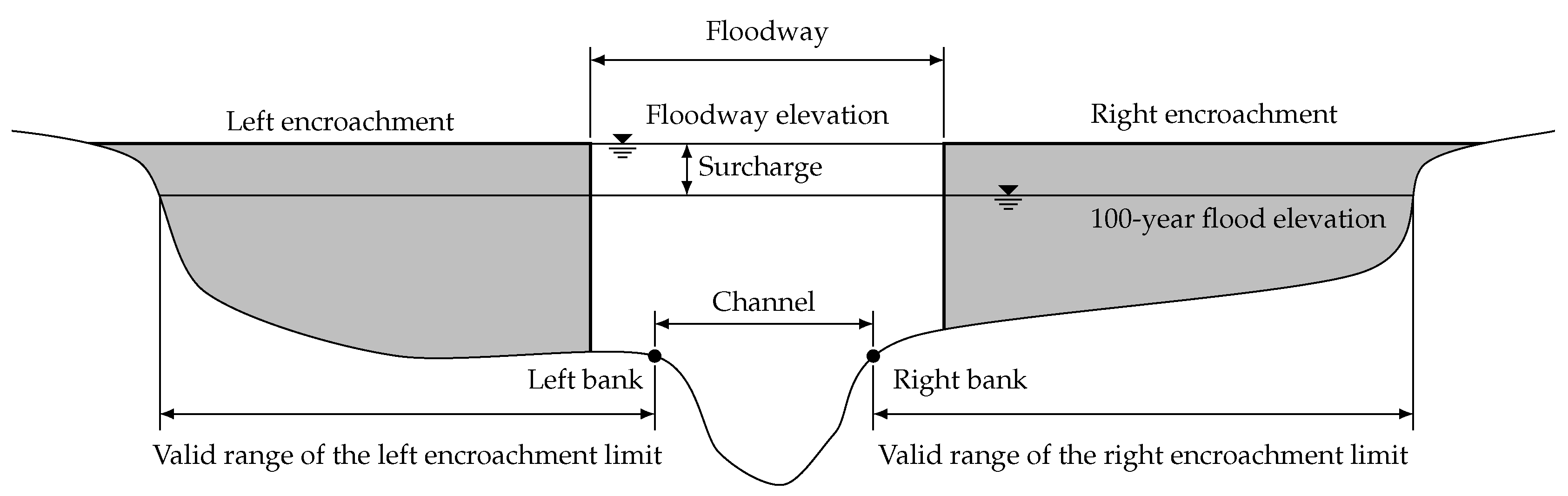
The floodway is defined by vertical encroachments on both sides of the main channel area within the 100-year floodplain as shown in Figure 1 and conveys flood water without raising the water surface elevation by a regulated threshold, typically set to be 0.305 m (1 ft) in the United States by FEMA unless a lesser rise criterion is imposed by the state [10]. Figure 1 shows a schematic of the 100-year flood elevation and the floodway elevation before and after encroachment, respectively. Ideally, development within the floodplain should be avoided. However, in dense urban areas, development that encroaches into the floodplain is unavoidable because an increase in human activities often pushes development closer to rivers and streams, and even into floodplains. At the same time, for safety reasons, many regulations do exist to prohibit excessive encroachments into natural streams because such encroachments can cause rise in the 100-year flood elevation and result in severe flooding upstream. The floodway then becomes a boundary to prevent encroachments from excessively impeding the conveyance of flow and hence excessive rise in the flood elevation. Since encroachment areas on both sides are often used for human activities such as business, leisure, parks, etc., it is one of the major interests for landowners and local governments to maximize these areas. To satisfy their interests in a safe manner, the width of the floodway can be reduced during flood modeling as long as the hydraulic requirements are met to minimize flood hazards. By optimizing the floodway, local governments can achieve more sustainable land use planning, better risk and safety assessment, and will be able to mitigate legal issues due to subjective floodway interpretations. However, floodway optimization is a difficult task because the floodway boundary can be established in many different ways [11].
Protocols in creating the floodway boundary are not well defined [12,13] and are primarily left to the practitioner [13]. One major problem without well-defined methods of floodway determination is that floodway boundaries produced by different modelers may vary significantly. Depending on the modeler’s motivation, experience level, and understanding of the subject matter, different modelers may produce different floodway boundaries even if given the identical hydraulic model. This subjectivity may not necessarily result in optimal floodway boundaries and hence highlights the need and advantage of a computer-aided optimization method.
Selvanathan and Dymond [14] developed an ArcGIS [15] tool that can run HEC-RAS, post-process the results, and visualize and smooth the floodway from within an ArcGIS environment. Their tool also allows the modeler to adjust encroachments visually inside ArcGIS and has a limited optimization routine that tries to satisfy the surcharge requirement. However, the focus of their research was mainly on automation of iterative HEC-RAS runs and post-processing of its outputs. Franz and Melching [11] introduced the Full Equations Utilities (FEQUTL) model that uses an iterative trial and error procedure to determine the left and right encroachment limits. Their model was not developed to perform reach-wide optimization of the floodway, but it does provide the reader with a glimpse of the technique used for floodway determination. Majority of focus in floodway modeling revolves around the criteria and methods used in floodway modeling [12,13,16,17]. Most discussions are primarily focused on modeling techniques, recommendations to modeling standards and procedures, and evaluating the practicality and feasibility of applying one uniform standard for all floodways. Thomas and Golaszewski [17] suggested an improved iterative procedure that involves a consideration of non-steady section-averaged velocity, variation of velocity-depth product, topographic and geomorphic features, control of hydraulic structures, flow conveyance and results of hydraulic models. They also acknowledged that an experienced practitioner is required to delineate and assess floodways using the improved iterative procedure.
Lots of effort in optimization of floodplains and floodways have been devoted towards the system operations of flow control structures within the floodway [18,19,20] and floodplain management related issues such as flood risk assessment and cost benefit analysis of different floods and structures [21,22,23,24,25,26,27,28,29,30,31]. Szemis et al. [18] introduced an optimization framework for scheduling environmental flow management alternatives using ant colony optimization [32]. Bogardi and Balogh [19] developed a model that calculates the probability of levee failures and optimizes floodway operations. Luke et al. [20] studied the impact on the floodway and levee damages in the New Madrid floodway in Missouri of the detonation control during May of 2011 and concluded that passive control would have greatly reduced the costs of repairing those hydraulic structures. Lund [21] used linear programming to develop an approach that minimizes the expected flood damages and costs. Shafiei et al. [22] examined different genetic algorithms (GA) [33] for optimizing the levee encroachment design and concluded that GAs are acceptable tools for solving the levee design problems while non-GA-based optimization techniques may not be able to find the global optimum of such problems because of the non-linear nature of the objective function surface. Mori and Perrings [23] developed a model for finding optimal floodplain development decisions. Yazdi and Neyshabouri [24] used the non-dominated sorting GA to find the optimal Pareto solutions of two objective functions minimizing flood mitigation costs and potential damages to the floodplain. Lu et al. [25] proposed an inexact sequential response planning approach for optimal management of floodplains. Porse [26] used linear programming to evaluate decisions for urban floodplain development and assess potential flood damages. Woodward et al. [27,28] developed a decision support system that generates effective mitigation measures and optimizes their performance using a multi-objective optimization algorithm. Lopez-Llompart and Kondolf [29] and Kondolf and Lopez-Llompart [30] studied how floodways in the Mississippi River had been affected by land use conflicts and management. Czigáni et al. [31] used the MIKE 21 model [34] for multi-purpose floodway zoning and floodway delineation along the lower Hungarian Drava section. However, very little has been done to produce an optimized floodway boundary for the entire stream [35] and an extensive literature review revealed Froehlich’s [36] and Yu’s [35] works.
Froehlich [36] suggested that delineation of the floodway boundary be done in a fair way. He pointed out legal issues including violation of the constitution with floodplain regulations and related those issues towards a need for a just and fair way to delineate a floodway. He further hinted that a reach-wide optimal solution would be an impartial way to define regulatory floodway boundaries. Froehlich’s proposed approach uses dynamic programming to delineate the floodway boundary of the steady-state energy balance equation using the standard step method. His research is significant in the way that he realized the importance of reach-wide optimization of the floodway and attempted to use dynamic programming as an optimization tool. However, since the work was done using hydraulic code that is not approved by FEMA, his floodway optimization technique cannot be used to generate floodplains and floodways for FEMA.
Yu [35] used a GA to calculate the floodway encroachment limits within HEC-RAS. For the objective function, he used the sum of the absolute difference of simulated and desired water surface elevations within the floodway for all cross sections. He attempted to find floodway encroachment limits that keep the surcharge for all cross sections within an acceptable range, but he did not consider minimizing the floodway area nor maintaining a subcritical flow state reach-wide. His approach was not able to produce better results than the default methods in HEC-RAS, but the idea of using a heuristic algorithm to determine the floodway aligns well with this study.
In one-dimensional riverine modeling, cross sections are extracted from terrain data along the river where there are hydraulically important features. For each cross section, the left and right encroachment limits are assigned, which define the floodway boundaries. In flood modeling, the flood elevations are interrelated between cross sections. When modeling streams that consist of only a few cross sections, it may be feasible to manually find optimal encroachment limits based on engineering judgments, but as the number of cross sections increases, seeking feasible floodway boundaries becomes more complex and time-consuming. This difficulty usually discourages the modeler from repeatedly running the model using different combinations of encroachment limits to determine the best feasible reach-wide solution that would meet the surcharge and hydraulic requirements. Even if the modeler is willing to put forth the trial and error effort, the floodway determined in this manner may not be optimized. Further, there is no one structured and uniform procedure that exists in defining the floodway area [12,13,16], let alone finding the best feasible one. The default methods built in HEC-RAS are generally used as a starting point [13] and should not be considered a method for reach-wide optimization. Optimization of the floodway in a reach-wide manner involves generating the left and right encroachment limits in each cross section that will result in a regulatory rise in the water surface elevation along the entire stream. At the same time, these encroachment limits should satisfy certain requirements set by the modeler. As we mentioned above, our interest is to minimize the footprint area of the floodway to maximize the land use of both encroachments by local governments while ensuring the hydraulic safety from potential flood hazards.
In this study, we developed software using the HECRASController to communicate with HEC-RAS and implemented an optimization method for reach-wide floodway determination using a heuristic algorithm called Isolated-Speciation-based Particle Swarm Optimization (ISPSO) [37] and the HEC-RAS hydraulic model. In Section 2, we defined the floodway optimization problem and formulated engineering judgments as an objective function to remove any subjectivity. We also briefly introduced ISPSO, and combined the objective function and ISPSO to elaborate on the development of the proposed method called the Automated Floodway Optimizer for HEC-RAS (AFORAS). In Section 3, we conducted a case study using a universally available floodway model from HEC-RAS and discussed its results. Finally, in Section 4, we highlighted the main advantages and limitations of AFORAS and concluded this study with a consideration of future work.
2. Materials and Methods
2.1. Study Area
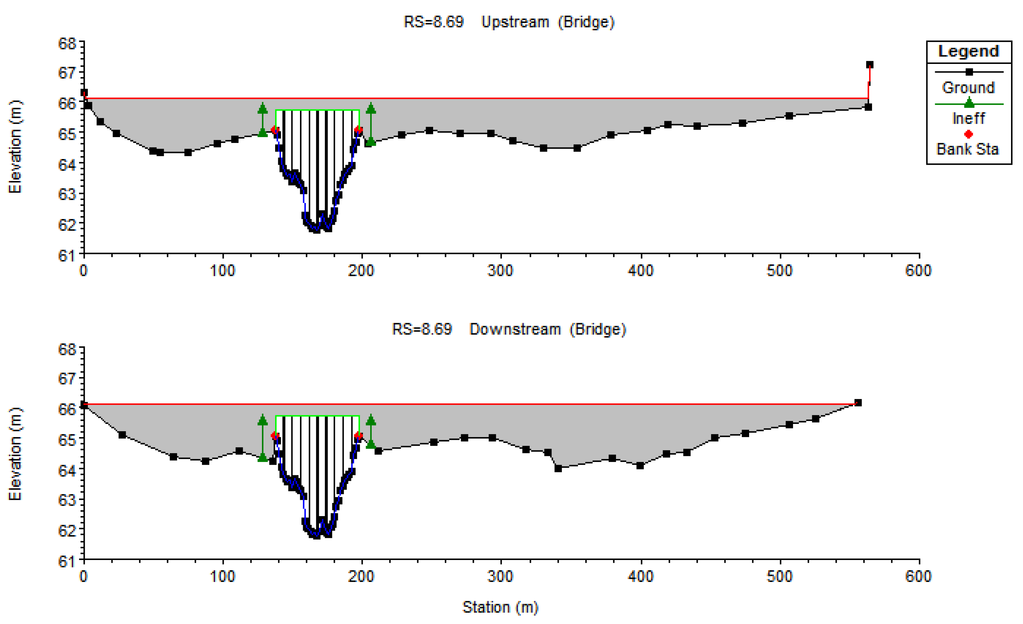
A floodway model called FLODENCR included in the HEC-RAS 4.1.0 installation was used for this study. This model was chosen at random to demonstrate the effectiveness of the optimization method. In addition, since input files for the case study are freely available from the HEC-RAS installation, researchers may duplicate the simulation if desired. Although this case study may not generalize all other cases, it serves as a simple but yet applicable case scenario where the floodway can be obtained using the optimization method and manually for cross-validating if the optimization method is indeed providing results that mimic the behavior of a manually obtained floodway. This model represents a 1.59 km of Beaver Creek near Kentwood, Louisiana, and consists of total 12 cross sections with a bridge structure as shown in Figure 2. Figure 3 shows the 9-pier bridge structure on Highway 1049 located at 8.69 km. The upstream area of the bridge is mostly covered by grass while its downstream area is dominated by forests. Two cross sections just upstream and downstream of the bridge define the geometries of the upstream and downstream faces of the structure, respectively. The opening under the low chord of the bridge is 60.05 m wide and its deck is 12.19 m wide. On both sides of the opening, ineffective areas are defined to model the embankment area that effectively blocks the water.
2.2. Mathematical Representation of the Problem
In order to optimize the floodway in HEC-RAS using an optimization algorithm, an objective function needs to be defined that evaluates the fitness of the model parameters objectively because there cannot be the modeler’s intervention during an optimization run. The objective function should reflect the modeler’s knowledge about the model and their engineering judgments about the model outputs.
Figure 4 depicts a floodway in a river with cross sections, channel banks, and 100-year floodplain extents. The hatched polygon representing the floodway is created by connecting the left and right encroachment limits in each cross section. The area of the hatched polygon indicates the floodway footprint area denoted by Afw in this section. In a similar way, the maximum and minimum floodway areas (Afw,max and Afw,min, respectively) can be calculated by connecting the 100-year floodplain extents (diamonds) and channel banks (dots), respectively. Our interest is to minimize the floodway area Afw while satisfying hydraulic requirements.
In floodway determination, the objective function should consider three criteria: (1) Floodway surface area, (2) surcharge, and (3) flow state indicating whether or not the flow is subcritical. The floodway surface area should be minimized while the surcharge is kept within acceptable limits and the subcritical flow state is maintained. There are many different hydraulic parameters in HEC-RAS. However, both models for the 100-year floodplain and floodway are required to share the same hydraulic parameters including the channel bottom geometry, Manning’s roughness coefficient, structural parameters, etc. because hydraulic modeling for the floodway should simulate the same hydraulic conditions as for the 100-year floodplain. Otherwise, the floodway model would not simulate the 100-year flood condition anymore. The only exception is the left and right encroachment limits which defines the floodway area. In other words, the optimization algorithm only adjusts the shape of the hatched polygon in Figure 4 and evaluates the model outputs to calculate the objective function. The model outputs from HEC-RAS provide the surcharge and cross-sectional Froude number [38], which can be used to evaluate violations of criteria (2) and (3) stated above. Ideally, the surcharge should be between 0 and an allowable limit mandated by the FEMA or the state government while the Froude number should be less than 1 for flow to be subcritical.
Most of the streams in the United States flow at a subcritical state except in the mountainous area, which is most likely undeveloped and underpopulated. Since FEMA only requires the floodway analysis for developed communities, the objective function in this study is formulated to handle subcritical flow conditions. However, if the flow state changes to supercritical, the modeler would have to choose the flow condition to model within HEC-RAS. In cases where the flow turns from subcritical to supercritical, HEC-RAS will default to the critical depth [2] to proceed with its calculation even though the water surface elevation may be erroneous. There are options within HEC-RAS for simulation of mixed-type or supercritical flows, but either the trial-and-error method or a priori knowledge of the flow state is required to be able to select these options. While the optimization algorithm itself does not discriminate between the different flow states, encroaching a stream that is flowing at a critical or supercritical flow state will, most often than not, result in a decrease in the water surface elevation and an excessive increase in the flow velocity. Since a negative surcharge is not allowed by FEMA [39], encroachment analysis is not necessary for the supercritical flow state in most of the case.
There are also two constraints: (1) The floodway should not be narrower than the area defined by the left and right channel banks because it should not affect the effective flow conveyance of the channel; and (2) the floodway limits cannot fall outside the 100-year floodplain by definition. The first constraint reserves the channel area between the left and right channel banks to carry the flood water by not impeding this area by floodway encroachment. The second constraint does not allow the floodway encroachment limits on a non-inundated dry area, which effectively leads to no encroachment at all in the river. In Figure 4, the left encroachment limit is constrained between the left channel bank (dots) and the left extent of the 100-year floodplain (diamonds). The same constraints apply to the right encroachment limit. These valid ranges of the left and right encroachment limits are shown in the cross-sectional view in Figure 1. From these two constraints, the minimum and maximum floodway bounds can be defined so that the objective function can compare different floodways by evaluating how close solutions are to the minimum possible floodway area. Given that the above two hydraulic conditions including the surcharge and Froude number are satisfactory, the floodway with the minimum surface area is deemed the optimal floodway.
By formulating the above three criteria and two constraints, the following objective function can be defined: otherwise
where is a parameter sample in a normalized hypercube search space , is the problem dimension, n is the number of cross sections to optimize, is a mapping function that maps a parameter sample to encroachment limits , which the HEC-RAS model takes as its input parameters to compute and , is the HEC-RAS model, is the objective function, Afw is the floodway surface area, Afw,min and Afw,max are the minimum and maximum surface areas of the floodway, respectively as shown in Figure 4, and are the surcharge and Froude number vectors, respectively, for all cross sections, and are the surcharge and Froude number, respectively, for cross section i, and N is the total number of cross sections in the model including n cross sections to optimize and those used as boundary conditions.
If the surcharges and Froude numbers of all cross sections ( and , respectively) are within acceptable ranges, the objective function evaluates the ratio of the surface area difference between the current and minimum floodways (Afw and Afw,min, respectively) to the surface area difference between the maximum and minimum floodways (Afw,max and Afw,min, respectively). Provided that all the hydraulic conditions are satisfied, the values of this ratio are 0 and 1 when the floodway is at its minimum and maximum widths, respectively. If one or more of the hydraulic conditions are violated, the objective function is set to unity and extra penalties are added based on how severely the surcharge and Froude number are deviating from their respective allowable limits. The penalty functions are designed so that the magnitude of deviation from the intended surcharge range or Froude number range is directly correlated to the magnitude of penalty added to the objective function. Any penalty will force the objective function to take on a larger value, which is an undesirable trait in a minimization problem. Now, floodway optimization is defined as a mathematical equation that can be evaluated objectively by computer code. The main goal of the proposed approach is to minimize the objective function by optimizing the variable vector that represents encroachment limits , using a heuristic algorithm.
To better explain how the objective function works, Table 1 shows example outputs from a simple hypothetical model and their objective function values in the Equation (1) column as well as Yu’s objective function values in the Equation (2) column. This hypothetical model consists of two cross sections (). Its minimum and maximum floodway areas are 50 km2 and 100 km2, respectively. Trial 1 evaluates the minimum floodway area, but the surcharges and Froude numbers for both cross sections violated hydraulic conditions (i.e., and for ). Since there are hydraulic violations, the penalty case of Equation (1) is used to calculate the objective function value in the Equation (1) column. That is, f (M(g(x))) = 1 + max(0 − 0.366/0.305, 0) . Similarly, trials 2–3 have some violations and use the same equation to evaluate the objective function. Trial 4 does not violate any hydraulic conditions, so the acceptable case of Equation (1) is used to calculate the objective function value. In this case, . Similarly, trials 5–6 do not have any violations and use the same floodway area ratio as their objective function values. Assuming that there are no more trial simulations, trial 4 would be the best floodway model because it minimizes the floodway area while satisfying all hydraulic requirements. In actual optimization runs, trials will evolve based on a heuristic algorithm introduced in Section 2.3.
For comparison, Yu’s objective function [35] is defined as:
This lump-sum way of integrating absolute differences can be problematic because bad performance in some cross sections with a high surcharge can be compensated for in other cross sections with a low surcharge. This compensation prohibits Equation (2) from differentiating good trials from bad ones. For example, both cross sections in trial 3 violated the surcharge requirement (i.e., for ) while the two cross sections in trial 4 did not (i.e., for ). However, Equation (2) evaluates to 0.07 for both trials. As shown above, this objective function cannot adequately rank different trials for better optimization because information about individual cross sections gets lost. At the same time, since this objective function evaluates surcharges closer to the maximum allowed limit (i.e., m) favorably, trials with lower surcharges are penalized even if they are actually more desirable. For example, trial 6 with both surcharges at the maximum evaluates to 0.00 while trial 5 with lower surcharges evaluates to 0.50. In the end, populations in a GA will evolve towards the limit and the surcharge requirement can easily be violated when the surcharge is too close to the allowed limit.
2.3. Isolated-Speciation-Based Particle Swarm Optimization
Isolated-Speciation-based Particle Swarm Optimization (ISPSO) [37] is a multi-modal heuristic optimization algorithm based on collective intelligence of individual particles in a swarm. In ISPSO, parameter samples are referred to as particles, which are collectively called a swarm. They fly around the parameter space and form multiple species based on spatial proximity. Individual particles keep track of their experience and share information with neighbors in the same species. Their velocities and next positions are determined by combining their private experience and neighbors’ experience. In this way, particles in one species converge to a local solution. Since there are multiple species in the search space, particles are able to find multiple local solutions, possibly including the global solution as well. More details about how this optimization algorithm works, mathematical examples, and a practical engineering problem can be found in [37].
Unlike gradient-based techniques, heuristic optimization algorithms do not depend on nor require local slope evaluation of the objective function surface. Since the HEC-RAS model transforms model inputs and parameters to model outputs non-linearly, the objective function surface may not be smooth and can be very complicate. Because of this complicate nature of the objective function surface, it becomes important to avoid dependency on the landscape gradient of the objective function surface to prevent solution finding algorithms from falling into inferior local pits. Particles in ISPSO are able to find multiple solutions in different regions of the search space without getting trapped into such inferior pits. For this reason, ISPSO has successfully been applied to stochastic rainfall generation [40,41,42,43], storm tracking [44], uncertainty analysis [45,46], and climate change studies [47,48]. The current version of ISPSO is implemented in the R language [49], which was also used to evaluate the objective function and run the HEC-RAS program.
2.4. Automated Floodway Optimizer for HEC-RAS
The Automated Floodway Optimizer for HEC-RAS (AFORAS) is a tool that automatically optimizes the floodway in a HEC-RAS model using ISPSO. The system is unique in that the modeler need not make manual adjustment trying different combinations of encroachment limits until an acceptable solution is found. For fully automating the optimization procedure, the Application Programming Interface (API) of HEC-RAS was used to interface the HEC-RAS program and ISPSO’s R code. A command-line program called the Command-Line Interface for HEC-RAS (CLIRAS) was developed to control the HEC-RAS program from an R environment. CLIRAS can change HEC-RAS plans, read cross section information such as river stations, bank stations, encroachment stations, flood extents, etc., update encroachment stations, and, finally, execute the HEC-RAS program. These features of CLIRAS are essential in controlling the HEC-RAS program without manual user interventions and for the ISPSO R code to be able to execute the HEC-RAS model for a specified number of times non-interactively. ISPSO executes CLIRAS internally to update and run the HEC-RAS model and extract results from it to evaluate the objective function.
AFORAS integrates the ISPSO R code, CLIRAS, and HEC-RAS as shown in Algorithm 1. The maximum number of iterations itermax tells ISPSO the total number of iterations to perform for optimization. The maximum number of HEC-RAS model runs is defined by itermax times the swarm size S (itermax × S). The HEC-RAS model is represented by M(·) and requires that two plans be defined: (1) 100-year floodplain and (2) floodway. The boundary conditions specify how the downstream or upstream end of the floodway should tie into adjacent existing floodways. There are four possible boundary conditions: (1) No existing floodways at the upstream and downstream ends of the study reach (BC = None), (2) floodway only at the downstream end (BC = DS), (3) floodway only at the upstream end (BC = US), and (4) floodways at both ends (BC = Both). The boundary conditions fix the encroachment limits at the most upstream, downstream or both cross sections, and therefore the problem dimension can be determined based on the number of cross sections and the number of boundary conditions. For example, when there are no upstream or downstream floodways to tie into (BC = None), all cross sections should be optimized, whereas the number of cross sections to optimize reduces by either 1 or 2 if one boundary condition (either BC = DS or BC = US) or two boundary conditions (BC = Both) are specified, respectively. The number of cross sections to optimize is indicated by n and the problem dimension is the total number of left and right encroachment limits on those n cross sections, which is . The recommended swarm size of [50] was used.
| Algorithm 1 Pseudocode for automated floodway optimization for HEC-RAS. | |
| Require: itermax | ▹ Maximum number of iterations |
| Require:M(·) | ▹ HEC-RAS model with 100-year and floodway plans and profiles |
| Require: BC ∈ {None, DS, US, Both} | ▹ Boundary conditions for the encroachment limits |
| Extract cross section information from M(·) | |
| Number of cross sections | |
| Number of boundary conditions | |
| ▹ Problem dimension | |
| ▹ Swarm size | |
| Afw,min, Afw,max ← Minimum and maximum possible areas of the floodway | |
| X number of D-tuples randomly sampled from | ▹ Initial population |
| Let that maps particles to encroachment limits | |
| iter | |
| repeat | ▹ ISPSO loop |
| for do | |
| Xi ← Row i from X | ▹ trial encroachment limits or particle i in ISPSO |
| Simulate M(g(Xi)) using CLIRAS | ▹ Execute the HEC-RAS program |
| Evaluate f (M(g(Xi))) | ▹Equation (1) |
| if or f (M(g(Xi))) < f (M(g(Xbest))) then | ▹ If Xi is better than Xbest |
| Xbest ← Xi | ▹ Store the best encroachment limits from the current iteration |
| end if | |
| end for | |
| if iter = 1 or f (M(g(Xbest))) < f (M(g(xbest))) then | ▹ If Xbest is better than xbest |
| xbest ← Xbest | ▹ Store the best encroachment limits so far |
| end if | |
| Evolve X using ISPSO | ▹ Evolution of the swarm in ISPSO |
| iter ← iter + 1 | |
| until iter = itermax or other conditions are satisfied | |
| Optimized encroachment limits (xbest) | ▹ Found the best encroachment limits |
The valid ranges of the floodway encroachment limits vary from cross section to cross section as shown in Figure 4 (dot–diamond). As can be seen in Figure 1 and Figure 4, even for the same cross section, the left and right encroachment limits can have different scales. Because our objective is to find the best feasible left and right encroachment limits, the problem space is constructed from D encroachment limits. However, different scales in different encroachment limits highly skew the problem space, which can negatively affect the performance of optimization. To address this issue, the problem space is normalized to using a mapping function . The mapping function is defined such that it transforms a particle (i.e., a trial set of normalized encroachment limits) in a hypercube search space back to a D-tuple of encroachment limits , which is a direct input to the HEC-RAS model . The particle at the lower limits of all dimensions (i.e., for ) defines the minimum possible floodway (dashed polygon in Figure 4) determined by the bank stations (dots in Figure 4) while the particle at the upper limits (i.e., for ) defines the maximum possible floodway (unfilled solid polygon in Figure 4) determined by the 100-year floodplain extents (diamonds in Figure 4). In other words, bank stations are mapped to while 100-year floodplain extents are mapped to . In this way, the floodway is guaranteed to be wider than the main channel such that the conveyance of flow is not highly obstructed. At the same time, the floodway cannot be wider than the 100-year floodplain. Floodway areas including the minimum and maximum areas Afw,min and Afw,max, respectively, are calculated by straightening the reach and calculating the area of the polygon defined by the bank stations for Afw,min or the 100-year floodplain extents for Afw,max. These minimum and maximum floodway areas Afw,min and Afw,max, respectively, are used in the objective function in Equation (1) to assess the fitness of the floodway defined by trial encroachment limits g(Xi). Once the problem is defined, ISPSO initializes the swarm and starts evolving the particles by evaluating trial encroachment limits. The final solution (xbest) is a set of optimized left and right encroachment limits, which then becomes input for the HEC-RAS floodway model.
2.5. Numerical Experiments
Three different approaches of producing the floodway were compared: (1) automated optimization by AFORAS, (2) manual determination by the authors, and (3) the default floodway in the model as a reference. For fair comparisons, the model was not modified except that floodway encroachment limits were updated. To update floodway encroachment limits using Algorithm 1, the mapping function is defined to normalize encroachment limits in the HEC-RAS model into . To define the mapping function , the bank stations and 100-year flood extents were extracted and normalized to create a unit hypercube search space where D is two times the number of cross sections to be optimized. After each iteration of evolution in Algorithm 1, particles in the problem space are transformed back to actual floodway encroachment limits, which are in turn input into the HEC-RAS model for evaluating the objective function in Equation (1).
The number of cross sections to be optimized varies depending on the boundary condition. Four encroachment boundary conditions as defined in Section 2.4 were tested: (1) BC = None, (2) BC = DS, (3) BC = US, and (4) BC = Both. The upstream-most and downstream-most encroachment limits of the default floodway in the reference model were used as those encroachment boundaries that an optimized floodway is to be tied into. Only in this way, the default model need not be updated at all and can be used as a reference model for the other two approaches.
Numerical experiments were conducted using the floodway model to observe how AFORAS performs in different boundary conditions. A total of 30 independent runs of each boundary condition were performed. Based on Clerc’s suggestion [50] and the number of dimensions in this problem, the recommended swarm size of 18 was used for the boundary condition BC = Both while 19 was used for the other three boundary conditions. For each AFORAS run, total 1000 iterations were performed resulting in total 18,000 and 19,000 model runs for the boundary condition BC = Both and the other boundary conditions, respectively.
3. Results and Discussion
3.1. Comparison of Different Approaches
The first AROFAS run for each boundary condition was used to compare the floodways between the three approaches. Table 2 shows the problem dimensions and the objective function values of the final floodways for the three approaches and four boundary conditions. The objective function value for the HEC-RAS floodway remains the same because its floodway was used as a reference and was not independently optimized. Since floodway optimization is a minimization problem, a floodway with the least objective function value is preferred. As can be seen in Table 2, among all the AFORAS floodway runs, the case with BC = Both yielded the worst objective function value (0.338), it but still performed better than the best floodway from the other two approaches (0.342). The numbers inside parentheses show that AFORAS reduced the objective function value by 1–29% from the manual method and by 12–40% from the HEC-RAS method. In terms of the floodway area, these numbers indicate the reduction of the floodway area outside the channel (Afw − Afw,min, not the total floodway area (Afw). On average for all eight cases (i.e., manual and HEC-RAS cases), the reduction of the floodway area outside the channel was 20%, which can significantly increase encroachment areas for development.
Despite high problem dimensions from 20 to 24, AFORAS performed reasonably well and even outperformed the manual optimization. An interesting observation is that the performance improved as the problem dimension increased with more cross sections to optimize. When either the upstream-most or downstream-most cross section of the floodway is specified as a boundary condition, the fixed width of the encroachments in those cross sections prevents the floodway area from being further reduced beyond its boundary condition limits.
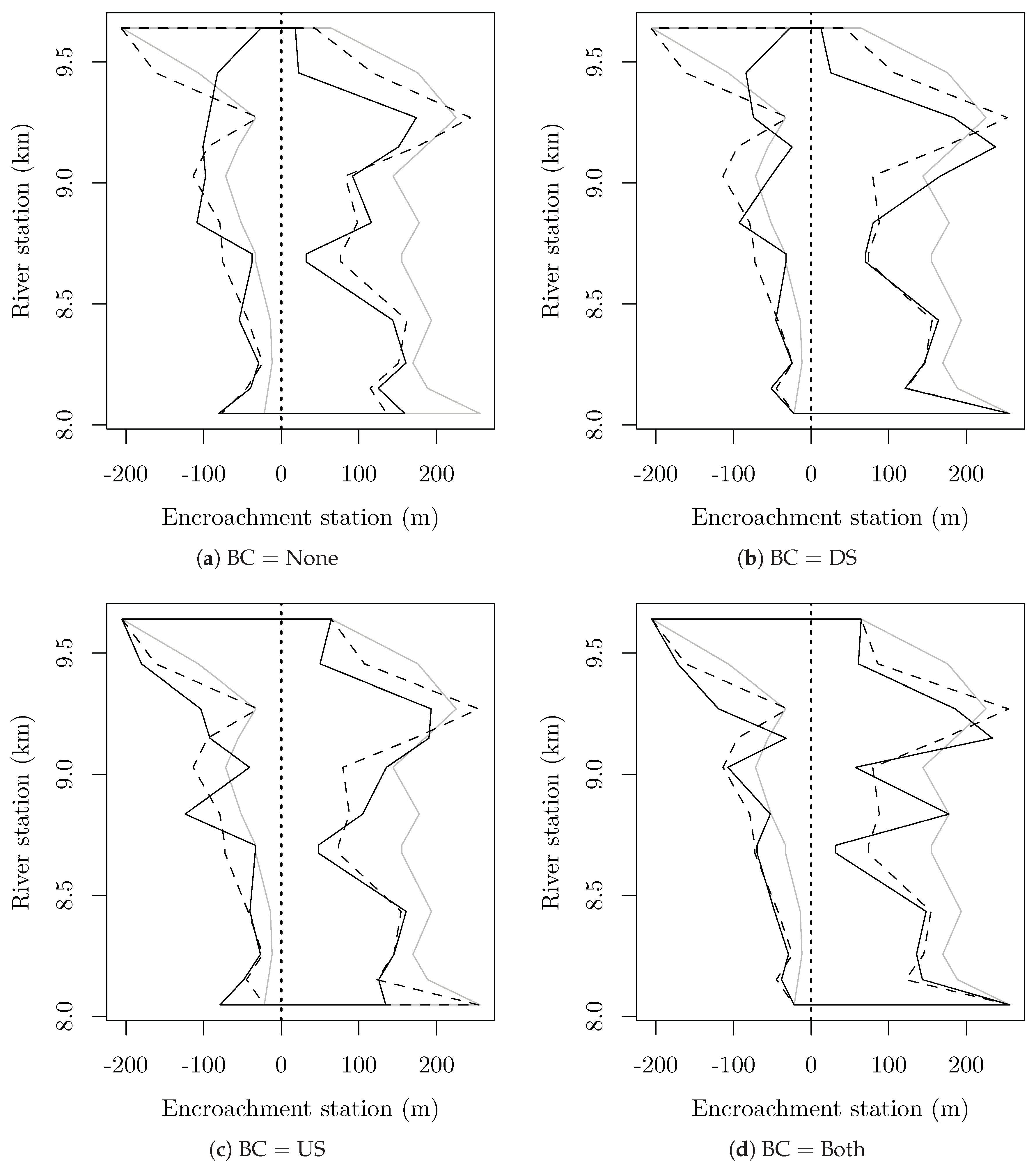
Figure 5 shows the final floodway for all cases with different boundary conditions. Vertical lines at encroachment station 0 represent the straightened river while negative and positive stations represent the left and right floodway encroachment limits on both sides of the river. For the case with BC = None, at the downstream-most cross section at river station 9.66 km, the floodway is narrower than those of the cases that have a restriction to the same cross section as a boundary condition (i.e., BC = DS and BC = Both). Similarly, for the case with BC = None, at the upstream-most cross section at river station 8.05 km, the floodway is narrower than those of the cases with BC = DS and BC = Both. Since these boundary conditions affect the objective function, lower objective function values in the BC = None case do not necessarily mean that AFORAS performs better when there are no boundary conditions specified. However, this result shows that AFORAS was able to take full advantage of cross sections that are not constrained to help reduce the footprint of the floodway and performed consistently better than the other two approaches.
3.2. Sensitivity of Encroachment Limits to the Boundary Condition
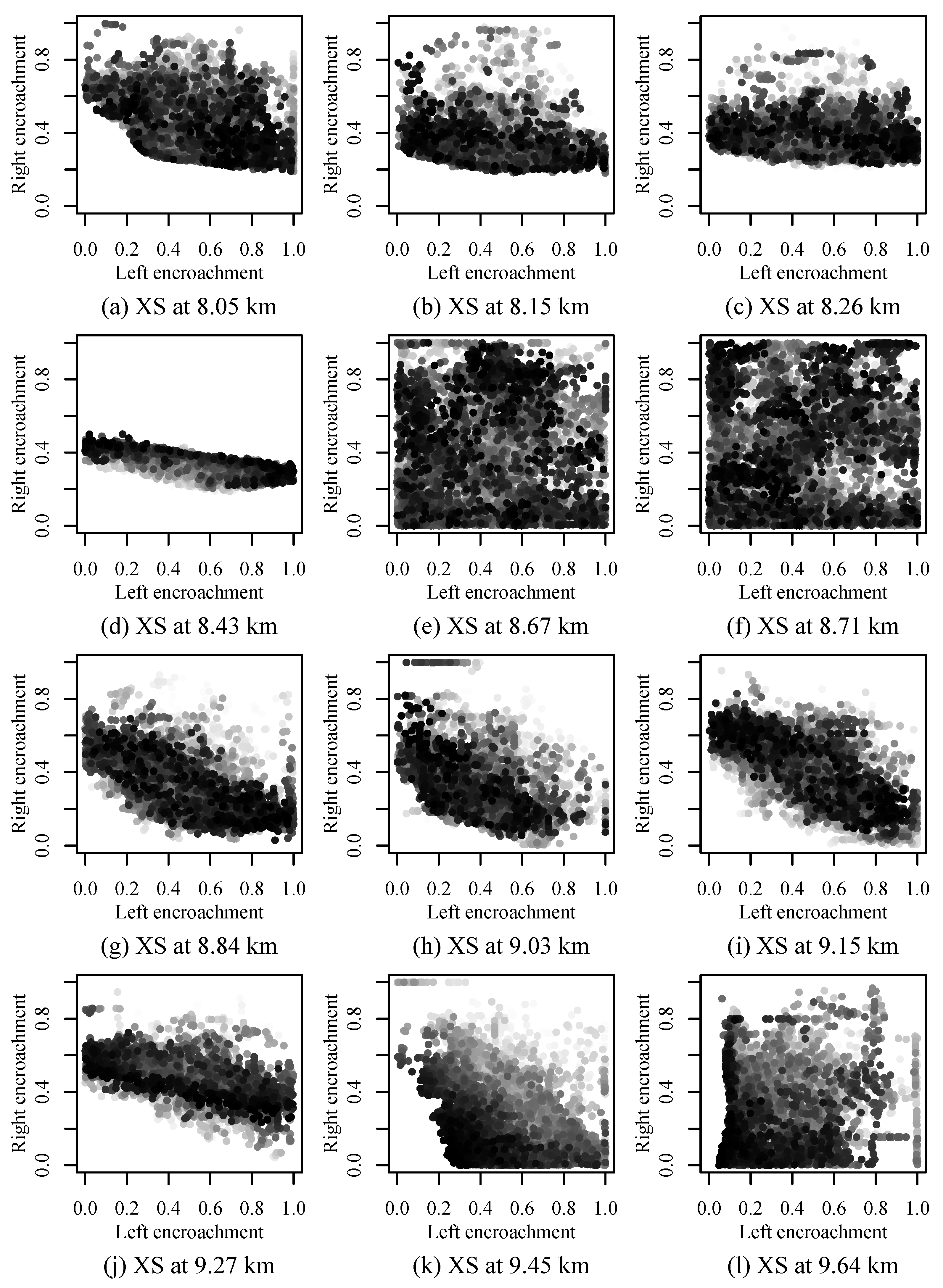
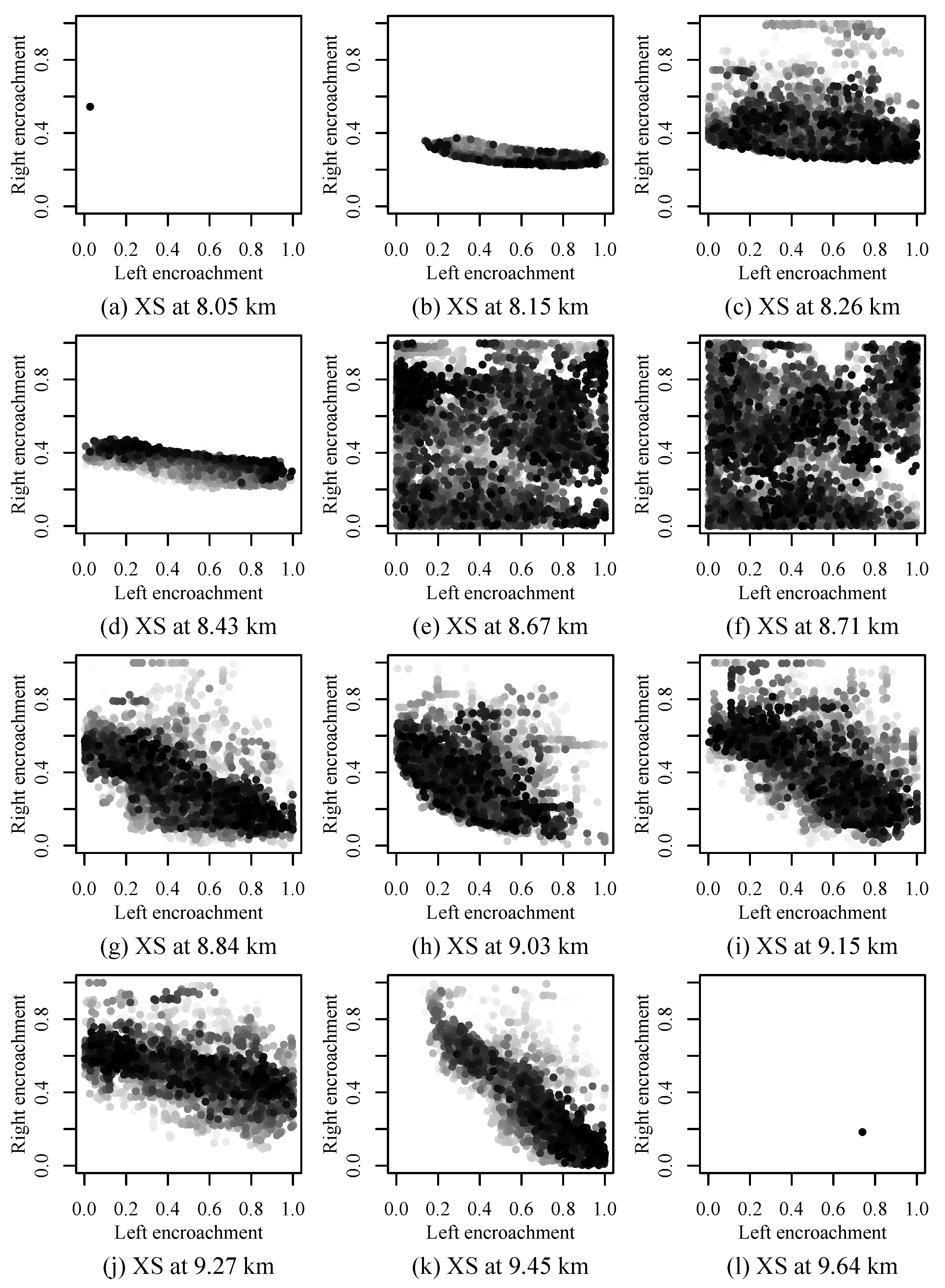
In optimization, it is beneficial to visualize the landscape of the objective function surface to be able to understand a problem. However, since most of floodway optimization problems deal with more than one cross section, their problem dimensions are usually higher than two, which makes it difficult to visualize the objective function surface without projecting it onto a much smaller-dimensional space. Figure 6 and Figure 7 show two-dimensional projections of 10,000 particles with grayscaled objective function values satisfying hydraulic requirements for BC = None and BC = Both, respectively. These plots show how sensitive particles were to the performance of optimization. The more spread out particles are along one encroachment limit, that encroachment limit was less sensitive to the performance because particles did not converge to a narrower band of the dimension. For example, in Figure 6e,f, particles tend to spread out almost randomly across the entire projected space. This widespread presence of particles means that they did not have any preference over specific encroachment limits in these cross sections at 8.67 km and 8.71 km during optimization and they were very insensitive to the performance compared to those in the other cross sections. Ideally, AFORAS should be able to take advantage of this insensitivity of particles to the performance of floodway encroachments in these two cross sections. The result of BC = None in Figure 5a (the very first run for this boundary condition) shows this behavior where AFORAS decided to take very narrow floodway encroachments as the final solution at these two cross sections. Since a bridge is located between these cross sections, ineffective flow areas were established around the bridge structure to model embankment areas. The areas immediately before and after the structure prevent the water from flowing freely downstream and result in ineffective flow areas. As a result, floodway encroachments within these ineffective flow areas could not affect the flood elevation significantly because those areas blocked by the floodway encroachments were already ineffective.
As shown in Figure 6a–d,g–k, in other cross sections except the upstream-most cross section, particles spread out more along the left encroachment axis than along the right encroachment axis. The narrow distribution of particles in the right encroachment axis means that the right encroachment limit was more sensitive to the performance and played a bigger role than the left encroachment limit during optimization. This result can be explained by the relative width of possible encroachment areas on the left overbank versus those on the right overbank. As shown in Figure 2, the portions of cross sections on the left side of the river line (i.e., left overbanks) are much narrower than those on the right side (i.e., right overbanks), especially at the downstream area. Because the encroachment widths on both overbanks are normalized to create a unit hypercube search space, wide-spread particles across the left encroachment do not necessarily mean that the left overbank area is wider. Also, for the same reason, significant movements of particles along the left encroachment dimension only slightly affect actual changes in the encroachment width, effectively making the left encroachment insensitive to the performance. However, since the left overbank gradually expands as it traverses upstream, this effect started slowly diminishing from 8.84 km.
The upstream-most cross section in Figure 6l showed a similar pattern to those around the bridge structure at 8.67 km and 8.71 km. Its insensitivity to the performance is due to the fact that HEC-RAS computes the flood elevation from downstream to upstream. Since the flood elevation within the floodway encroachment at the upstream-most cross section does not affect any downstream flood elevations, encroachment limits at this cross section may be placed anywhere as long as the hydraulic criteria are satisfied. For AFORAS, this insensitivity means that it should pick the narrowest possible floodway, which can be seen in the result in Figure 5. What it also means is that the problem with BC = None can be simplified by constraining the encroachment limits in the upstream-most cross section to the bank stations and solving the problem as if it had the boundary condition BC = US. In this way, the problem dimension of BC = None can be reduced by two and AFORAS should be able to achieve better performance and a faster convergence rate.
Two-dimensional plots for the boundary conditions BC = DS and BC = US are not presented in this paper because of space limitations and a prohibitively large number of data points. However, cross sections from 8.26 km to 9.27 km in these boundary conditions showed similar patterns to Figure 6c–j or Figure 7c–j. Cross sections at 8.05 km and 8.15 km in the boundary condition BC = US behaved similarly to Figure 6a,b, respectively (i.e., both cases do not constrain the downstream-most cross section). Also, cross sections at 9.45 km and 9.64 km in the boundary condition BC = DS behaved similarly to Figure 6k,l, respectively (i.e., both cases do not constrain the upstream-most cross section).
When the downstream-most cross section is constrained (i.e., BC = DS or BC = Both), the right encroachment became even more sensitive to the performance at 8.15 km, just upstream of the downstream boundary cross section, and its encroachment plot for BC = DS is very similar to Figure 7b. This neighbor cross section was highly affected by the downstream boundary condition because of the backward calculation of HEC-RAS. When the upstream-most cross section is constrained (i.e., BC = US or BC = Both), AFORAS was able to achieve faster convergence by avoiding unnecessary trial-and-error sampling in the upstream-most cross section, which does not affect any other cross sections at all. The encroachment plot for 9.45 km, just downstream of the upstream boundary condition, became much narrower than Figure 6k with most particles clustering around the diagonal line from top-left to bottom-right as shown in Figure 7k. Table 3 summarizes these observations of two-dimensional projection subplots of all particles from 30 AFORAS runs.
3.3. Optimization Performance
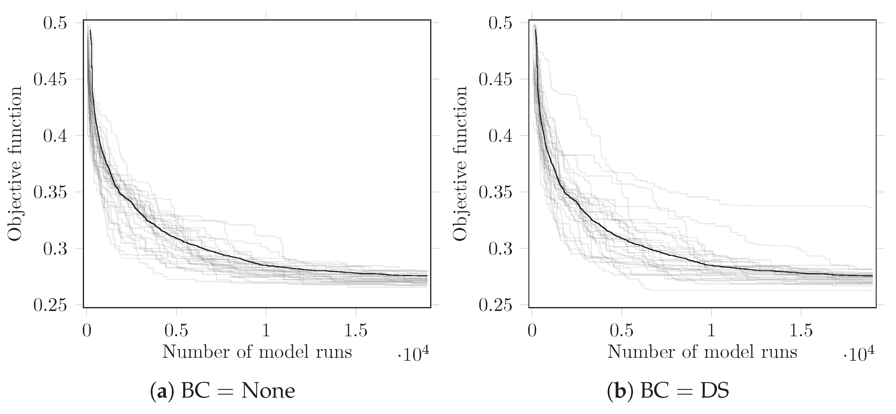
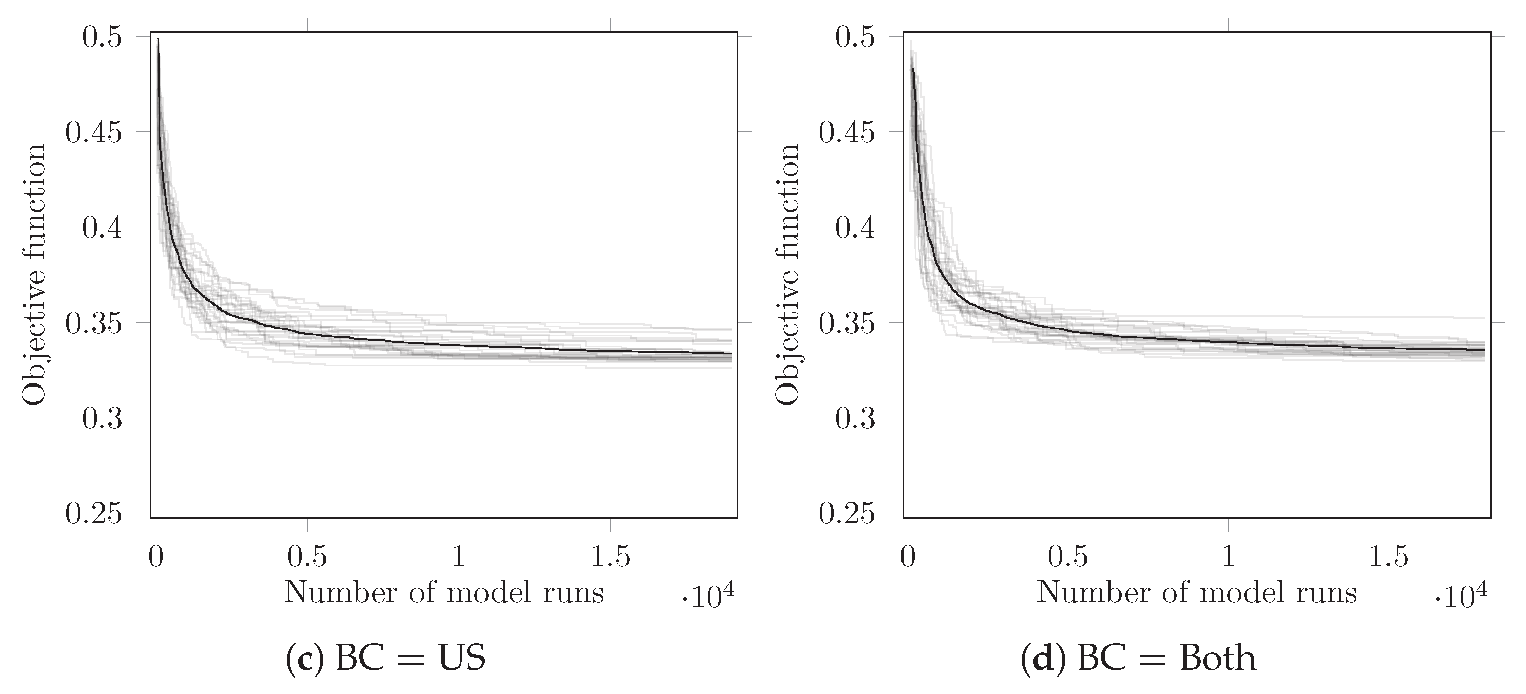
The convergence lines of all 30 AFORAS runs for different boundary conditions are presented in Figure 8 as 30 gray lines with the average performance as a black line. All the runs converged exponentially to the final values of the objective function. The minimum and maximum of the final values are 0.265 and 0.280, respectively, and their mean and standard deviation are 0.272 and 0.004, respectively. The standard deviation is approximately 1.5% of the mean, which indicates that the performance of AFORAS is very robust and reliable. The black line shows the mean of the 30 cumulative minimum values of the objective function. The average performance converges very quickly until 5000 model runs and experiences gradual improvement until about 15,000 model runs for BC = None and BC = DS, and 10,000 model runs for BC = US and BC = Both, after which the convergence rate slowed down significantly. Figure 8 shows that AFORAS achieved a faster convergence rate for the cases where the upstream-most cross section is constrained as a boundary condition. However, their objective function values are higher or worse than those for the other two cases. The higher objective function values for BC = US and BC = Both is because the upstream-most cross section used as a boundary condition is fairly wide compared to the bank stations, which act as the lower limits in that cross section for the other cases. Particles in BC = None and BC = DS where the upstream-most cross section was also optimized, found a very narrow floodway width at this cross section as the final solution. On the other hand, this cross section was fixed at a much larger width as a boundary condition for BC = US and BC = Both and produced worse objective function values. Since the two sets of boundary conditions have different search spaces, the higher objective function values do not necessarily mean poor performances.
3.4. AFORAS as a Tool for Floodway Optimization
To the authors’ knowledge, Yu’s study [35] was the first attempt to determine the floodway encroachment limits using HEC-RAS and a GA, but his approach did not consider the floodway area and subcritical flow state. Also, as we compared our objective function to his in Section 2.2, the lump-sum way of integrating information across all cross sections leads to information loss and a lack of differentiation between good and bad models. AFORAS takes a different approach for floodway determination by taking into account the flow state and minimizing the floodway area. At the same time, its objective function is formulated to separate out favorable models from those with hydraulic violations.
AFORAS integrates ISPSO and HEC-RAS for reach-wide optimization of the floodway area. The derivative- free search of ISPSO and a mathematical representation of floodway area optimality were integrated as AFORAS in a way that HEC-RAS can be executed automatically by computer code without user interventions. AFORAS was successful in seeking and improving the floodway encroachment limits for the case study. As discussed above, AFORAS was able to identify those cross sections that are insensitive to its performance and almost fully encroached the floodway at these locations so that the floodway area was kept to the minimum. Overall, AFORAS performed consistently better than the manual approach and the reference floodway, and showed reliable and consistent performance across different boundary conditions. It is also interesting to see that ISPSO, as a heuristic algorithm, is able to reliably solve high dimensional problems in this study. As summarized in Table 2, the problem dimension for this study varied from 20 to 24. Different problem dimensions result in different landscapes of the objective function, but, as shown in Figure 6 and Figure 7, two-dimensional projections onto individual cross sections of the objective function surface exhibit similar patterns depending on which cross section was used as a boundary condition. Despite the differences in the surface of the objective function and its final values, convergence was achieved for all cases and the solutions found by AFORAS minimized the floodway area while keeping the surcharge and flow state within the allowable limits. These observations suggest that AFORAS can be a suitable tool for reach-wide floodway optimization.
While AFORAS can be a good candidate for reach-wide floodway optimization, it is only limited to handle reaches with subcritical flows. The proposed objective function within AFORAS has to be modified to accommodate cases with mixed or supercritical flows, which are not as common as subcritical flows already handled by AFORAS. More tests are needed to observe the performance of ISPSO given a different objective function that can handle varying flow states. Also, when calculating the floodway area, AFORAS currently assumes that the river line is straight and the floodway encroachment limits vary linearly between consecutive cross sections. While this simplification of geometries may be a reasonable assumption for optimization, a more realistic evaluation of the floodway area can be attained by incorporating the natural curvature of the river line. Finally, a sensitivity analysis needs to be performed to see how the numbers of particles and iterations for an ISPSO run affect the performance of AFORAS and find the right balance between computing time and the performance. Better a priori estimation of the total number of model runs may help reduce computing time. Future work and research on AFORAS will include addressing these limitations and running more HEC-RAS floodway models with different geometries and structures.
4. Conclusions
Since the floodway is an essential part of hydrologic and hydraulic studies of riverine flooding, in the United States, FEMA requires one to be determined for developed communities using their approved computer programs, one of which is HEC-RAS. HEC-RAS has widely been used for flood risk and floodway regulation studies by many researchers. Because the floodway encroachment area is often used for human activities, it is a local government’s interest to expand this area by minimizing the floodway footprint area that conveys the flood water without affecting the water surface elevation too much. Our objective is to minimize the floodway area while maintaining the surcharge and subcritical flow state reach-wide, both of which are required by FEMA. The authors’ literature review has revealed that very little work has been done in terms of floodway optimization. A recent attempt to determine the floodway encroachment limits using HEC-RAS and a GA did not consider the floodway area and subcritical flow state, which most of the streams in the United States exhibit. The proposed objective function takes into account the floodway area, surcharge, and subcritical flow state to make sure that the final optimized floodway not only meets FEMA’s hydraulic requirements but also maximizes floodway encroachment areas for human activities in a reach-wide manner. By integrating the objective function and a heuristic algorithm called ISPSO, we proposed a floodway area optimization tool named AFORAS for reach-wide optimization of the floodway using HEC-RAS. We used a readily and freely available floodway model from the HEC-RAS 4.1.0 installation for a case study so that other researchers can replicate our results if they decide. Comparisons of the AFORAS, manual, and HEC-RAS approaches showed 1–40% improvements in the objective function value by AFORAS. AFORAS consistently provided superior results for all the boundary conditions. We also conducted a sensitivity analysis of encroachment limits to the boundary condition and a convergence test by running AFORAS 30 times for four different boundary conditions. Both left and right encroachment limits were insensitive to the performance in cross sections adjacent to a bridge structure while these encroachment limits exhibited different level of sensitivity to the performance in other cross sections. Because of the bridge opening and ineffective areas, encroaching these cross sections could not affect the flood elevation much and did not help improve the objective function compared to the other cross sections. The surface of the objective function may vary significantly for different HEC-RAS models or even for different combinations of the boundary conditions in the same floodway model. In this regard, it is advantageous for AFORAS to employ ISPSO over gradient-based optimization techniques because of the capability of ISPSO to solve high dimensional problems without requiring the derivative of the objective function. Limitations in the current AFORAS method include the lack of support for mixed and supercritical flows in the objective function, and the linear approximation of the river geometry and floodway. Also, since the total number of HEC-RAS runs has to be specified a prior, a quantitative analysis would be beneficial to reduce computing time by estimating how many model runs are required in advance. Addressing these limitations and recommending the required number of model runs a prior will be left for research in the near future.
Author Contributions
Conceptualization, T.M.Y.; Methodology, H.C. and T.M.Y.; Software, H.C.; Validation, T.M.Y., H.C. and J.H.; Formal Analysis, T.M.Y. and H.C.; Investigation, T.M.Y.; Resources, J.H.; Data Curation, H.C.; Writing—Original Draft Preparation, H.C., T.M.Y. and J.H.; Writing—Review & Editing, H.C., T.M.Y. and J.H.; Visualization, H.C.; Supervision, T.M.Y.; Project Administration, T.M.Y.; Funding Acquisition, N/A.
Funding
This research received no external funding.
Conflicts of Interest
The authors declare no conflict of interest.
References
- FEMA. Guidance for Flood Risk Analysis and Mapping: General Hydrologic Considerations. 2018. Available online: https://www.fema.gov/media-library-data/1525201756728-390e667d3d0958347b8374f6321bd488/General_Hydrologic_Guidance_Feb_2018.pdf (accessed on 18 April 2018).
- FEMA. Guidance for Flood Risk Analysis and Mapping: Hydraulics—One-Dimensional Analysis. 2016. Available online: https://www.fema.gov/media-library-data/1484864685338-42d21ccf2d87c2aac95ea1d7ab6798eb/Hydraulics_OneDimensionalAnalyses_Nov_2016.pdf (accessed on 28 December 2016).
- Brunner, G.W. HEC-RAS River Analysis System User’s Manual Version 4.1; US Army Corps of Engineers, Institute for Water Resources, Hydrologic Engineering Center: Davis, CA, USA, 2010. [Google Scholar]
- Rastislav, F.; Martina, Z. The HEC-RAS model of regulated stream for purposes of flood risk reduction. Sel. Sci. Pap. J. Civ. Eng. 2016, 11, 59–70. [Google Scholar] [CrossRef]
- ShahiriParsa, A.; Noori, M.; Heydari, M.; Rashidi, M. Floodplain zoning simulation by using HEC-RAS and CCHE2D models in the Sungai Maka River. Air Soil Water Res. 2016, 2016, 55–62. [Google Scholar] [CrossRef]
- Golshan, M.; Jahanshahi, A.; Afzali, A. Flood hazard zoning using HEC-RAS in GIS environment and impact of Manning roughness coefficient changes on flood zones in semi-arid climate. Desert 2016, 21, 25–34. [Google Scholar]
- Balogun, O.S.; Ganiyu, H.O. Development of inundation map for hypothetical Asa dam break using HEC-RAS and ArcGIS. Arid Zone J. Eng. Technol. Environ. 2017, 13, 831–839. [Google Scholar]
- Ben Khalfallah, C.; Saidi, S. Spatiotemporal floodplain mapping and prediction using HEC-RAS-GIS tools: Case of the Mejerda River, Tunisia. J. Afr. Earth Sci. 2018, 142, 44–51. [Google Scholar] [CrossRef]
- Goodell, C. Breaking the HEC-RAS Code: A User’s Guide to Automating HEC-RAS; h2ls: Portland, OR, USA, 2014. [Google Scholar]
- FEMA. Flood Insurance Study Guidelines and Specifications for Study Contractors. 2002. Available online: http://www.fema.gov/media-library-data/20130726-1546-20490-8681/frm_scg.doc (accessed on 24 December 2015).
- Franz, D.D.; Melching, C.S. Full Equations Utilities (FEQUTL) Model for the Approximation of Hydraulic Characteristics of Open Channels and Control Structures During Unsteady Flow; Technical Report Water-Resources Investigations Report 97–4037; U.S. Department of the Interior, U.S. Geological Survey: Reston, Virginia, USA, 1997.
- Howells, L.; McLuckie, D.; Collings, G.; Lawson, N. Defining the floodway—Can one size fit all? In Proceedings of the 44th Annual Floodplain Management Australia Conference, Coffs Harbour, Australia, 12–14 May 2004. [Google Scholar]
- Thomas, C.R.; Honour, W.; Golasweski, R. Procedures for floodway definition: Is there a uniform approach? In Proceedings of the 50th Annual Floodplain Management Australia Conference, Gosford, Australia, 23–26 February 2010. [Google Scholar]
- Selvanathan, S.; Dymond, R.L. FloodwayGIS: An ArcGIS visualization environment to remodel a floodway. Trans. GIS 2010, 14, 671–688. [Google Scholar] [CrossRef]
- Esri. ArcGIS Desktop: Release 10; Esri: Redlands, CA, USA, 2011. [Google Scholar]
- Rigby, T. Floodplain development manual (NSW) A document in need of review. In Proceedings of the 47th Annual Floodplain Management Australia Conference, Gunnedah, Australia, 27 February–1 March 2007. [Google Scholar]
- Thomas, C.R.; Golaszewski, R. Refinement of procedures for determining floodway extent. In Proceedings of the 52nd Annual Floodplain Management Australia Conference, Batemans Bay, Australia, 21–24 February 2012. [Google Scholar]
- Szemis, J.M.; Maier, H.R.; Dandy, G.C. A framework for using ant colony optimization to schedule environmental flow management alternatives for rivers, wetlands, and floodplains. Water Resour. Res. 2012, 48. [Google Scholar] [CrossRef] [Green Version]
- Bogárdi, I.; Balogh, E. Flood system operation along levee-protected rivers. J. Water Resour. Plan. Manag. 2013, 140, 04014014. [Google Scholar] [CrossRef]
- Luke, A.; Kaplan, B.; Neal, J.; Lant, J.; Sanders, B.; Bates, P.; Alsdorf, D. Hydraulic modeling of the 2011 New Madrid Floodway activation: A case study on floodway activation controls. Nat. Hazards 2015, 77, 1863–1887. [Google Scholar] [CrossRef]
- Lund, J.R. Floodplain planning with risk-based optimization. J. Water Resour. Plan. Manag. 2002, 128, 202–207. [Google Scholar] [CrossRef]
- Shafiei, M.; Bozorg-Haddad, O.; Afshar, A. GA in optimizing Ajichai flood levee’s encroachment. In Proceedings of the 6th World Scientific and Engineering Academy and Society International Conference on Evolutionary Computing, World Scientific and Engineering Academy and Society, Lisbon, Portugal, 16–18 June 2005. [Google Scholar]
- Mori, K.; Perrings, C. Optimal management of the flood risks of floodplain development. Sci. Total Environ. 2012, 431, 109–121. [Google Scholar] [CrossRef] [PubMed]
- Yazdi, J.; Neyshabouri, S.S. A simulation-based optimization model for flood management on a watershed scale. Water Resour. Manag. 2012, 26, 4569–4586. [Google Scholar] [CrossRef]
- Lu, H.W.; He, L.; Du, P.; Zhang, Y.M. An inexact sequential response planning approach for optimizing combinations of multiple floodplain management policies. Pol. J. Environ. Stud. 2014, 23, 1245–1253. [Google Scholar]
- Porse, E. Risk-based zoning for urban floodplains. Water Sci. Technol. 2014, 70, 1755–1763. [Google Scholar] [CrossRef] [PubMed]
- Woodward, M.; Gouldby, B.; Kapelan, Z.; Hames, D. Multiobjective optimization for improved management of flood risk. JW Resour. Plan. Manag. 2014, 140, 201–215. [Google Scholar] [CrossRef]
- Woodward, M.; Kapelan, Z.; Gouldby, B. Adaptive flood risk management under climate change uncertainty using real ooption and optimization. Risk Anal. 2014, 34, 75–92. [Google Scholar] [CrossRef] [PubMed] [Green Version]
- Lopez-Llompart, P.; Kondolf, G.M. Encroachments in floodways of the Mississippi River and Tributaries Project. Nat. Hazards 2016, 81, 513–542. [Google Scholar] [CrossRef]
- Kondolf, G.M.; Lopez-Llompart, P. National-local land-use conflicts in floodways of the Mississippi River system. AIMS Environ. Sci. 2018, 5, 47–63. [Google Scholar] [CrossRef]
- Czigáni, S.; Pirkhoffer, E.; Halmai, A.; Lóczy, D. Application of MIKE 21 in a multi-purpose floodway zoning along the lower Hungarian Drava section. Revista de Geomorfologie 2016, 18, 5–18. [Google Scholar] [CrossRef]
- Dorigo, M.; Maniezzo, V.; Colorni, A. The ant system: Optimization by a colony of cooperating agents. IEEE Trans. Syst. Man Cybern. Part B Cybern. 1996, 26, 1–13. [Google Scholar] [CrossRef] [PubMed]
- Goldberg, D.E. Genetic Algorithms in Search, Optimization, and Machine Learning; Addison-Wesley: Boston, MA, USA, 1989. [Google Scholar]
- DHI. MIKE 21 FlowModel FM. Parallelisation Using GPU. Benchmarking Report. 2014. Available online: http://www.mikebydhi.com/~/media/Microsite_MIKEbyDHI/Publications/PDF/GPU_Benchmarking.ashx (accessed on 28 September 2018).
- Yu, L. Using Genetic Algorithms to Calculate Floodway Stations with HEC-RAS. Master’s Thesis, University of Dayton, Dayton, OH, USA, 2015. [Google Scholar]
- Froehlich, D.C. A fair way to a floodway: Optimal delineation of floodplain encroachment limits. In Proceedings of the 1999 Water Resources Engineering Conference, Seattle, WA, USA, 8–12 August 1999. [Google Scholar]
- Cho, H.; Kim, D.; Olivera, F.; Guikema, S.D. Enhanced speciation in particle swarm optimization for multi-modal problems. Eur. J. Oper. Res. 2011, 213, 15–23. [Google Scholar] [CrossRef]
- Chanson, H. Development of the Bélanger equation and backwater equation by Jean-Baptiste Bélanger (1828). J. Hydraul. Eng. 2009, 135, 159–163. [Google Scholar] [CrossRef]
- FEMA. Guidance for Flood Risk Analysis and Mapping: Floodway Analysis and Mapping. 2016. Available online: https://www.fema.gov/media-library-data/1484864412580-de4aa11166f23a8f06e6121925a5b543/Floodway_Analysis_and_Mapping_Nov_2016.pdf (accessed on 28 December 2016).
- Kim, D.; Olivera, F.; Cho, H. Effect of the inter-annual variability of rainfall statistics on stochastically generated rainfall time series: Part 1: Impact on peak and extreme rainfall values. Stoch. Environ. Res. Risk Assess. 2013, 27, 1601–1610. [Google Scholar] [CrossRef]
- Kim, D.; Olivera, F.; Cho, H.; Lee, S.O. Effect of the inter-annual variability of rainfall statistics on stochastically generated rainfall time series: Part 2: Impact on watershed response variables. Stoch. Environ. Res. Risk Assess. 2013, 27, 1611–1619. [Google Scholar] [CrossRef]
- Kim, D.; Olivera, F.; Cho, H.; Socolofsky, S. Regionalization of the modified Bartlett-Lewis rectangular pulse stochastic rainfall model. Terr. Atmos. Ocean. Sci. 2013, 24. [Google Scholar] [CrossRef]
- Kim, D.; Cho, H.; Onof, C.; Choi, M. Let-It-Rain: A web application for stochastic point rainfall generation at ungaged basins and its applicability in runoff and flood modeling. Stoch. Environ. Res. Risk Assess. 2016, 31, 1023–1043. [Google Scholar] [CrossRef]
- Cho, H.; Kim, D.; Lee, K.; Lee, J.; Lee, D. Development and application of a storm identification algorithm that conceptualizes storms by elliptical shape. J. Korean Soc. Hazard Mitig. 2013, 13, 325–335. [Google Scholar] [CrossRef]
- Cho, H.; Olivera, F. Application of multimodal optimization for uncertainty estimation of computationally expensive hydrologic models. J. Water Resour. Plan. Manag. 2014, 140, 313–321. [Google Scholar] [CrossRef]
- Cho, H.; Kim, D.; Lee, K. Efficient uncertainty analysis of TOPMODEL using particle swarm optimization. J. Korean Water Resour. Assoc. 2014, 47, 285–295. [Google Scholar] [CrossRef]
- Heo, J.; Yu, J.; Giardino, J.R.; Cho, H. Impacts of climate and land-cover changes on water resources in a humid subtropical watershed: A case study from East Texas, USA. Water Environ. J. 2015, 29, 51–60. [Google Scholar] [CrossRef]
- Heo, J.; Yu, J.; Giardino, J.R.; Cho, H. Water resources response to climate and land-cover changes in a semi-arid watershed, New Mexico, USA. Terr. Atmos. Ocean. Sci. 2015, 26. [Google Scholar] [CrossRef]
- R Development Core Team. R: A Language and Environment for Statistical Computing; R Foundation for Statistical Computing: Vienna, Austria, 2006; ISBN 3-900051-07-0. Available online: http://www.r-project.org (accessed on 9 November 2015).
- Clerc, M. Standard Particle Swarm Optimization. 2012. Available online: http://clerc.maurice.free.fr/pso/SPSO_descriptions.pdf (accessed on 24 December 2013).
Figure 1.
Schematic of the 100-year flood elevation and floodway.

Figure 2.
River and cross section geometries for Beaver Creek near Kentwood, Louisiana, in the FLODENCR model. The arrow indicates the direction of flow. A bridge structure is located at 8.69 km.
Figure 2.
River and cross section geometries for Beaver Creek near Kentwood, Louisiana, in the FLODENCR model. The arrow indicates the direction of flow. A bridge structure is located at 8.69 km.

Figure 3.
Bridge structure on Highway 1049 located at 8.69 km.

Figure 4.
Plan view of a floodway along with a river, cross sections, channel banks, and 100-year floodplain extents.
Figure 4.
Plan view of a floodway along with a river, cross sections, channel banks, and 100-year floodplain extents.

Figure 5.
Graphical views of the left and right encroachment limits for the four different boundary conditions. Vertical lines at encroachment station 0 represents the river line. Negative and positive stations represent the left and right encroachment limits, respectively. ![Water 10 01420 i001]() Straightened river,
Straightened river, ![Water 10 01420 i002]() Automated Floodway Optimizer for HEC-RAS (AFORAS) floodway,
Automated Floodway Optimizer for HEC-RAS (AFORAS) floodway, ![Water 10 01420 i003]() Manual floodway, and
Manual floodway, and ![Water 10 01420 i004]() Hydrologic Engineering Center’s River Analysis System (HEC-RAS) floodway.
Hydrologic Engineering Center’s River Analysis System (HEC-RAS) floodway.
 Straightened river,
  Automated Floodway Optimizer for HEC-RAS (AFORAS) floodway,
  Manual floodway, and
  Hydrologic Engineering Center’s River Analysis System (HEC-RAS) floodway.
Figure 5.
Graphical views of the left and right encroachment limits for the four different boundary conditions. Vertical lines at encroachment station 0 represents the river line. Negative and positive stations represent the left and right encroachment limits, respectively. ![Water 10 01420 i001]() Straightened river,
Straightened river, ![Water 10 01420 i002]() Automated Floodway Optimizer for HEC-RAS (AFORAS) floodway,
Automated Floodway Optimizer for HEC-RAS (AFORAS) floodway, ![Water 10 01420 i003]() Manual floodway, and
Manual floodway, and ![Water 10 01420 i004]() Hydrologic Engineering Center’s River Analysis System (HEC-RAS) floodway.
Hydrologic Engineering Center’s River Analysis System (HEC-RAS) floodway.
Straightened river, Automated Floodway Optimizer for HEC-RAS (AFORAS) floodway, Manual floodway, and Hydrologic Engineering Center’s River Analysis System (HEC-RAS) floodway.
Figure 6.
Two-dimensional projections of all particles Xi for satisfying the three hydraulic criteria from all 30 AFORAS runs for BC = Both. Since the total number of particles meeting hydraulic requirements was excessively large—130,395 out of 570,000 ()—10,000 particles were sampled to construct each subplot, which represents one cross section (XS). Particles that perform better are plotted darker in front of those that perform worse and are in a lighter gray.

Figure 7.
Two-dimensional projections of all particles Xi for satisfying the three hydraulic criteria from all 30 AFORAS runs for BC = None. Since the total number of particles meeting hydraulic requirements was excessively large—142,937 out of 540,000 ()—10,000 particles were sampled to construct each subplot, which represents one cross section (XS). Particles that perform better are plotted darker in front of those that perform worse and are in a lighter gray.

Figure 8.
Cumulative minimum values of the objective function vs. the number of model runs. The gray lines and black line represent 30 runs of AFORAS and the mean of those runs, respectively.
Figure 8.
Cumulative minimum values of the objective function vs. the number of model runs. The gray lines and black line represent 30 runs of AFORAS and the mean of those runs, respectively.


Table 1.
Example model outputs and their objective function values. For all trials, , Afw,min = 50 km2, and Afw,max = 100 km2.
Table 1.
Example model outputs and their objective function values. For all trials, , Afw,min = 50 km2, and Afw,max = 100 km2.
| Trial | (m) | (m) | Violations | Equation (1) | Equation (2) | |||
|---|---|---|---|---|---|---|---|---|
| 1 | 50 | 0.366 | 0.397 | 1.1 | 1.2 | 4 | 1.80 | 0.50 |
| 2 | 60 | 0.336 | 0.366 | 1.0 | 0.8 | 3 | 1.30 | 0.30 |
| 3 | 70 | 0.310 | 0.320 | 1.1 | 0.9 | 1 | 1.17 | 0.07 |
| 4 | 80 | 0.295 | 0.295 | 0.9 | 0.7 | 0 | 0.60 | 0.07 |
| 5 | 90 | 0.244 | 0.214 | 0.8 | 0.6 | 0 | 0.80 | 0.50 |
| 6 | 100 | 0.305 | 0.305 | 0.9 | 0.8 | 0 | 1.00 | 0.00 |
Table 2.
Objective function values for the test cases with different boundary conditions. Since Automated Floodway Optimizer for HEC-RAS (AFORAS) solves a minimization problem, lower values represent better models. The numbers inside parentheses indicate what percent of the objective function value could be improved by running AFORAS.
| BC | Problem Dimension | AFORAS | Manual | HEC-RAS |
|---|---|---|---|---|
| None | 24 | 0.270 | 0.348 (29%) | 0.379 (40%) |
| DS | 22 | 0.278 | 0.345 (24%) | 0.379 (36%) |
| US | 22 | 0.333 | 0.347 (4%) | 0.379 (14%) |
| Both | 20 | 0.338 | 0.342 (1%) | 0.379 (12%) |
Table 3.
Summary of two-dimensional projection subplots of all particles by Figure 6 and Figure 7. A ∼ symbol indicates a similar pattern to the subplots given on the right. Figure 6c–j and Figure 7c–j, respectively, have a similar pattern.
| BC | XS 8.05 km | XS 8.15 km | XS 8.26 km–9.27 km | XS 9.45 km | XS 9.64 km |
|---|---|---|---|---|---|
| None | 5a | 5b | 5c–5j | 5k | 5l |
| DS | 6a | ∼6b | ∼5c–5j | ∼5k | ∼5l |
| US | ∼5a | ∼5b | ∼5c–5j | ∼6k | 6l |
| Both | 6a | 6b | 6c–6j | 6k | 6l |
© 2018 by the authors. Licensee MDPI, Basel, Switzerland. This article is an open access article distributed under the terms and conditions of the Creative Commons Attribution (CC BY) license (http://creativecommons.org/licenses/by/4.0/).
Share and Cite
MDPI and ACS Style
Cho, H.; Yee, T.M.; Heo, J. Automated Floodway Determination Using Particle Swarm Optimization. Water 2018, 10, 1420. https://doi.org/10.3390/w10101420
AMA Style
Cho H, Yee TM, Heo J. Automated Floodway Determination Using Particle Swarm Optimization. Water. 2018; 10(10):1420. https://doi.org/10.3390/w10101420
Chicago/Turabian StyleCho, Huidae, Tien M. Yee, and Joonghyeok Heo. 2018. "Automated Floodway Determination Using Particle Swarm Optimization" Water 10, no. 10: 1420. https://doi.org/10.3390/w10101420
Note that from the first issue of 2016, this journal uses article numbers instead of page numbers. See further details here.