
Optimization of Inventory Holding Cost Due to Price, Weight, and Volume of Items †


Austin E. Cofrin School of Business, University of Wisconsin-Green Bay, Green Bay, WI 54311, USA
†
An earlier version was presented at the 2019 Decision Sciences Institute Annual Conference, New Orleans, LA, USA.
J. Risk Financial Manag. 2021, 14(2), 65; https://doi.org/10.3390/jrfm14020065
Submission received: 11 December 2020
/
Revised: 22 January 2021
/
Accepted: 28 January 2021
/
Published: 4 February 2021
(This article belongs to the Section Mathematics and Finance)
Abstract
:The inventory carrying cost has been assumed uniform for all products in an organization or a warehouse. This assumption is not valid for a diversified range of items in an organization or warehouse. This paper tested this hypothesis of variations in inventory holding costs in a warehouse in two industries based on the physical nature and the price of products. It is found that organizations with a wide variety of products need to calculate the inventory holding cost for each item (SKU) rather than using an average percentage cost of inventory. Inventory holding costs of items in two different organizations were calculated based on the various factors, including the actual cost of space due to the voluminous nature of the items with their existing inventory policies. A variation in inventory holding costs for each item was observed. The variation was small for an organization with homogeneous input costs, and it was large for a multi-product organization. The overall savings in the inventory holding cost due to adjusting the inventory policies through this methodology was found to be about 3%, which is significant for a big organization. This analysis will affect the decision the determining inventory carrying cost, inventory policies (e.g., stocking levels), and pricing policies (e.g., quantity discounts) for retail organizations.
1. Introduction
Inventory management is needed for every organization. People manage inventories for small businesses intuitively and do not feel the need for analytical skills due to the small value of the inventories held in stores. The need to manage inventory scientifically is crucial for large organizations due to the value of the inventory. Inventory is the largest block of money in a manufacturing organization (Gurtu et al. 2015b, 2019). Inventory in organizations includes, but is not limited to, raw materials, finished goods, work-in-progress (WIP), consumables, and spare parts (Waters 2003, p. 9). Inventory items differ between organizations due to the nature of businesses, such as manufacturing, trading, and retail, and by type of industry such as automotive, healthcare, construction. Inventory and inventory holding costs are not the same across organizations, even in the same industry. Inventory items are different among organizations based on many factors such as industry, size of the operation, location, and lead-time, to name a few. For example, inventory items are different in an automotive organization, a restaurant, and a consulting organization. In other words, the needs for inventory management and the importance of items are not uniform across industries and organizations (Nagpal and Chanda 2021).
Maintaining inventory in manufacturing and retail organizations is a necessity for ensuring smooth operations. Keeping inventory in a store or warehouse has a cost termed as inventory holding cost or inventory carrying cost. The ideal situation is just-in-time (JIT) delivery, which eliminates keeping inventory and does not incur any holding inventory cost. However, this is not a practical solution for most manufacturing, trading, or retail organizations. Therefore, maintaining an optimal inventory is necessary for organizations. The phenomenon of optimizing lot size, considering inventory holding cost and set up cost for an item, was first discussed a century ago by Harris (1913). It has gone through many modifications that will be discussed in detail in the next section. Some authors have discussed multi-product supply chains using a single inventory holding cost (Bahl 1982; Balintfy 1964; Eilon 1959; Tantiwattanakul and Dumrongsiri 2019; Zhang 2009). The inventory holding cost varies between organizations and the locations (Ghasemkhani et al. 2019; Goodarzian et al. 2020). This variation is mainly due to the variation in the cost of space and finance cost. However, the inventory carrying cost is considered the same at one location for all items in an organization. A fixed-rate (%) is used for the average cost of holding inventory in academic literature and practice.
This paper questions the assumption to use an average cost of holding inventory for all the items in an organization at a location due to the space occupied by an item and draws some parallels from transportation. It is well known that the inventory holding cost can differ across items, e.g., perishables items or items requiring refrigeration have a much higher inventory holding cost than non-perishable items. Similarly, obsolescence cost also varies depending on the item. For example, fashion apparels have high obsolescence cost as compared to furniture. However, this paper studies the inventory holding cost due to the space occupied by items in two industries, requiring a refrigerated storage facility for its products and another requiring a non-refrigerated (non-perishable) storage facility for all its products. Inventory has two states—stationary and mobile. Inventory is stationary in stores and warehouses, and inventory is mobile during transportation. Mobile inventory is on semi-truck, ship, train, or plane. The cost of inventory in a mobile state, i.e., during transportation, is determined by cube out or weigh out. Cube out is the situation when a piece of equipment (container, ship, or truck) has reached its volumetric capacity while the permitted weight limit exists, e.g., whitegoods. On the other hand, weighing out is when a piece of equipment has reached its weight limit, but the space is available for adding more content, e.g., steel plates/rods. The storage of most of the items falls under the cube out condition.
A similar concept of costing is proposed for inventory in a stationary state, i.e., in a store or a warehouse. This concept will be explained in detail later in the paper. The inventory holding costs of various items as stock-keeping units (SKU) were analyzed for two organizations for validating this concept. One organization is a dairy product processing organization with a relatively homogenous cost of raw materials. Another organization is a trading organization for the various products used by dentists, which have a significant variation in the costs of items, price per unit weight, and price per unit volume. The analyses suggest that the holding cost of each item should be considered instead of using an average cost of holding inventory at each location of warehouses and stores.
This paper’s contribution is that it demonstrates a variation in inventory holding costs for items in an organization. These variations are significant for organizations manufacturing, trading, or retailing various items with different cost densities (explained later in the paper). Therefore, finance departments of organizations dealing with multiple products should evaluate the use of an average cost (%) of holding inventory. The rest of the paper is organized as follows. Section 2 provides a literature review followed. Section 3 describes the research procedure. Section 4 provides analyses of the inventory holding cost for items of the two organizations. Section 5 provides a numerical example and discusses the finding. Section 6 concludes the paper with a discussion on managerial implications, some limitations, and potential future expansions.
2. Literature Review
The phenomenon of optimizing lot size, considering inventory holding cost and set up cost, was first discussed a century ago by Harris (1913). Goyal (1977) introduced the first significant change in this model. Goyal (1977) considered coordination between a vendor and a manufacturer in determining the lot-size. The same concept can be used between a manufacturer and a retailer. In other words, Goyal’s model is for a two-echelon supply chain. The author took inventory holding costs and set up costs of a manufacturer and a vendor to determine the optimal cost of the lot. Ten years later, Banerjee (1986) refined this model with a lot for lot policy, i.e., manufacturing and shipment lots are the same. (Goyal 1988) further refined this model by decoupling the number of shipment-lots from a production lot, i.e., multiple shipments are sent from one manufacturing lot. A large number of authors have used the models of Banerjee (1986) and (Goyal 1988) to modify the constraints and design new policies (Aljazzar and Gurtu 2019; Arslan and Turkay 2013; Battini et al. 2014; Braglia and Zavanella 2010; Cárdenas-Barrón et al. 2020; Chen et al. 2013; Dhandapani and Uthayakumar 2016; Dobson et al. 2017; Gurtu et al. 2015a; Jaber et al. 2013; Khalilpourazari and Pasandideh 2016; Khan et al. 2014; Perera et al. 2017; Rajput et al. 2019; Rastogi et al. 2017; Santhi and Karthikeyan 2018; Sundara Rajan and Uthayakumar 2017; Wahab et al. 2011; Zahran et al. 2015). Readers may read the various quantitative models compiled by Jaber and Zolfaghari (2008) and the centennial issue of the International Journal of Production Economics on this topic edited by Cárdenas-Barrón et al. (2014) for more details.
However, all the papers on inventory management have considered a single holding cost or an average holding cost for a vendor, a manufacturer, or a retailer in two-echelon supply chains until this paper. A paper on inventory management of many spare parts also used a single inventory holding cost (Heinen and Hoberg 2019). Coordinated supply chains used a single inventory holding costs (Zissis et al. 2019). Chen et al. (2015) talked about dynamic pricing based on inventory holding cost as a linear function using a single inventory holding cost. The papers analyzing multi-product (Pasandideh et al. 2014) and multi-generation technology products (Nagpal and Chanda 2021) also considered a single value of inventory holding costs. Choi and Enns (2004) have used two different rates for work-in-progress and finished goods, where both the rates are dollars/unit/time, i.e., not linked to volume or weight of items. It is critical to clarify that coordinated inventory models use different inventory holding costs for different players involved. However, each player uses one inventory holding cost for all the items, whereas this paper suggests using different inventory holding costs for various items by each player.
Some evidence from logistics and transport literature is presented on how the cost is calculated during transit. Logistics organizations charge the cost of transportation based on volume with a limit to max weight in a container, trailer, or truck. A standard general-purpose container is twenty feet long. All containers are referred to as the equivalent of this size as TEU (Twenty-Foot Equivalent Unit). International Standard Organization governs the sizes, and a twenty-foot container code is 22G0 or 22G1 (CSI Containers Services International 2020). The gross weight and maximum payload of a twenty-foot container are 67,200 lb. and 62,150 lb. respectively (Container Alliance 2020). The difference between these two weights is the weight of an empty container. Shippers charge for the cost of a container subject to the above maximum weight limit. However, most of the containers do not carry full weight. The weight of containers shipped between the EU and Asian countries varies between 81.5 percent (max) and 55.7 percent (min) of the allowed weight. Ninety-six percent of the containers weigh less than 80 percent, and 64 percent of the containers weigh less than 50 percent of the max weight (Gurtu et al. 2017). Therefore, the cost of transportation for lighter items is higher than the cost of transportation for heavier items.
Despite these variations in the weight and area (or space) density of items, the inventory holding cost is considered uniform across items in an organization in a stationary state. This is reflected in academic papers and the current industry practice, as verified by the author with many supply chain management practitioners and managers in accounting and finance departments. Waters (2003, p. 59) has assumed the typical inventory holding cost to be around 20% of the item cost per year. Many authors have taken average inventory holding costs in the range of 16% to 20% per year (Aljazzar and Gurtu 2019; Banerjee 1986; Braglia and Zavanella 2010; Goyal 1977, 1988; Gurtu et al. 2015a). Thus, the use of a fixed cost of holding inventory for all items is a limitation of the existing literature and presents a research gap. This paper addresses this gap in the existing literature and examines the cost of holding inventory for items or categories (family) of items in an organization. The next section explains the research design and details of the categories of items.
3. Research Procedure
In the EOQ model, the overall cost is optimized using inventory holding costs and set up costs. Therefore, a change in inventory holding cost affects the economic order quantity (EOQ). Inventory holding cost is affected by many factors such as the cost of finance, inventory holding period, inventory levels (quantity), and cost of storage space, among others. The effects of the inventory holding period and quantity have been studied in detail, as discussed in the previous section. The effects of finance cost in two-echelon supply chains affected by payment period have been studied by Aljazzar et al. (2018). The cost of storage space due to the nature of products is studied in this paper.
The paper presents a new method of calculating inventory holding cost, which is used in EOQ. Therefore, for calculating the optimal lot size (EOQ) using the new inventory holding cost, the assumptions of classical EOQ are applicable, such as:
- The demand is constant over time.
- No shortages are allowed.
- All the costs, including the rate of financial cost of holding, will remain constant.
- The entire lot will be sent in a shipment
Many organizations deal with multiple products or product families. Some products have high value but occupy a small storage area (or space), e.g., jewelry, electronic items, and cosmetic products. Some have low value but occupy a large area (or space), e.g., tissue paper. There is a large variety of products (or product families) between these two extremes. Since the storage area required for different products varies, this will affect inventory holding costs. For this analysis, the stoke-keeping unit (SKU) has been used and referred to as an item. Steps followed for this analysis are:
- Identify if the analysis will be done at the level of each SKU or a representative SKU from the family of items.
- Find out storage location, storage bin/pallet size, number of units in each bin/pallet, how many bins/pallets are kept on a shelf (or ground), how many bins/pallets are kept over each other on a shelf (or ground).
- Based on the current average inventory, annual sale, unit price, lead time, space cost, and cost of finance, calculate the inventory holding cost for each of the SKUs.
- The sum of all the SKUs’ inventory holding costs must be equal to the average inventory holding cost.
These steps have been converted into an analytical formula for use in other organizations. The revised inventory holding cost is to be used for calculating the new EOQ using the existing formula. Hence, that is not discussed in this paper. The notations used for calculating inventory holding and validating the average cost of holding inventory are as follows:
| I | average annual inventory of a warehouse | $ |
| h | inventory holding cost at a warehouse | % |
| hw | annual average holding cost for all items in a warehouse | $ |
| Aw | area of a warehouse | Sq. ft. |
| Cw | rent of the empty warehouse | $ |
| α | area utilization factor for storage where 0 < α < 1 | % |
| Ai | area of a rack-type i (this is the area of the pallet that is stored on the ground) | Sq. ft. |
| Si | number of shelves in the racks of type i (for storage on the ground, N = 1) | Number |
| Bj | number of bins (or pallets) type j kept on a shelf | number |
| Xk | number of stock-keeping units (SKU) in a bin (or on a pallet) where k is an SKU | Number |
| Pk | unit price of an SKU k | $/unit |
| Ik | average annual inventory of SKU k | Number |
| Cf | annual cost finance for an organization at a location | % |
| Co | cost of obsolescence | % |
| Ch | cost of handling a bin/pallet | $/unit |
The storage area in a warehouse is less than the total area due to non-storage areas such as receiving docks, inspection areas, aisles, and equipment storage space. Therefore, the effective cost of storage is higher than the per square foot cost of an empty warehouse.
Usually, items are stored in bins or on pallets, and these bins and pallets are stored in racks. Only very bulky items are stored on the floor in a single high formation, for example, vehicles. Racks have sleeves, and each shelf contains multiple bins or pallets. It is assumed that one shelf does not contain multiple sizes of bins or a combination of bins and pallets to keep the calculations simple.
Each bin (or pallet) may have more than one stock-keeping unit (SKU). Therefore,
where the number of bins from Equation (3) must be rounded-up. The space cost of an SKU is calculated by multiplying Equations (1)–(3). It is important to remember to use the rounded-up value of Equation (3). Therefore,
Finance cost, obsolescence cost, and handling cost of holding inventory are given in Equations (5)–(8) as follows:
It is reiterated that the number of bins or pallets (Ik/Xk) in Equations (4) and (7) must be rounded-up. The total cost of holding inventory for an SKU in a warehouse is the sum of Equations (4)–(7) as follows:
The total cost of holding inventory for all the items in a warehouse is the summation of the holding cost for all the items given by Equation (8). This is represented as follows:
Further, variation in the holding cost for each SKU is calculated as the difference from the organization’s average cost of holding inventory. The inventory holding costs of the various items (SKU) for two organizations were analyzed using the above methodology. The formula in Equation (9) is generalized for ease of use by any organization. The methodology and numbers were validated using the formula . The calculated average inventory holding cost was found to be identical to the organization’s average inventory holding cost (h). This validation illustrated that using an average inventory holding cost will not highlight the problem of charging higher inventory cost to some products and lower to some other products because the average will still be the same. However, this does not mean that using an average is the right strategy. The process steps and analysis of the two organizations and the findings are discussed in the next section.
4. Analysis of Inventory in Organizations
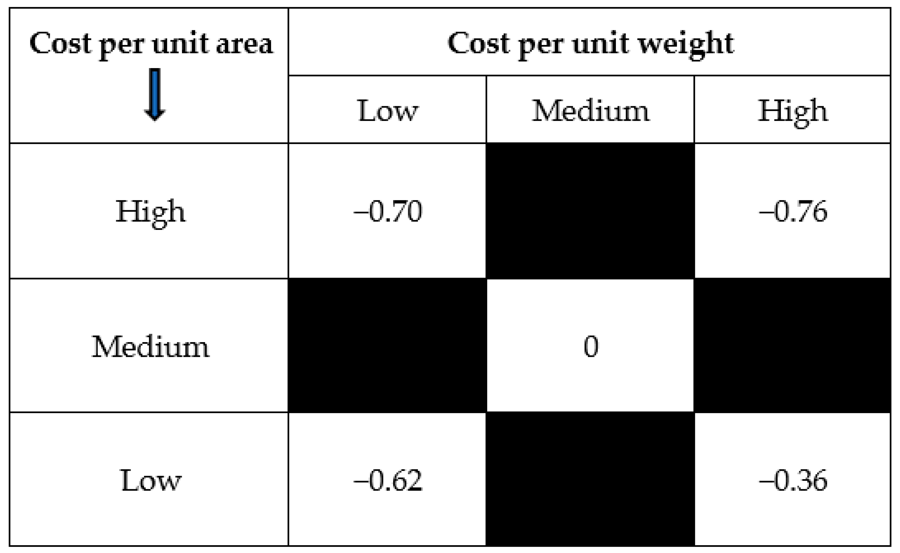
Inventory analysis of two organizations from two different industries was done. The first one will be referred to as A and the second one as B from now onwards. Organization-A is a dairy product processing organization. It is one of the largest cheese manufacturing organizations in the world. It has a relatively homogenous cost of raw materials. This organization’s final products have a small variation in its products’ unit price per unit area. Therefore, its products were categorized into five families of products, as shown in Figure 1, and a representative product from each family was selected for analysis. The SCM leaders from each organization identified these five representative products. Organization-A has multiple warehouses with variations in technologies/automation used. The analysis was done for one of the warehouses. Nevertheless, the cost of holding inventory at other locations is very likely to be different.
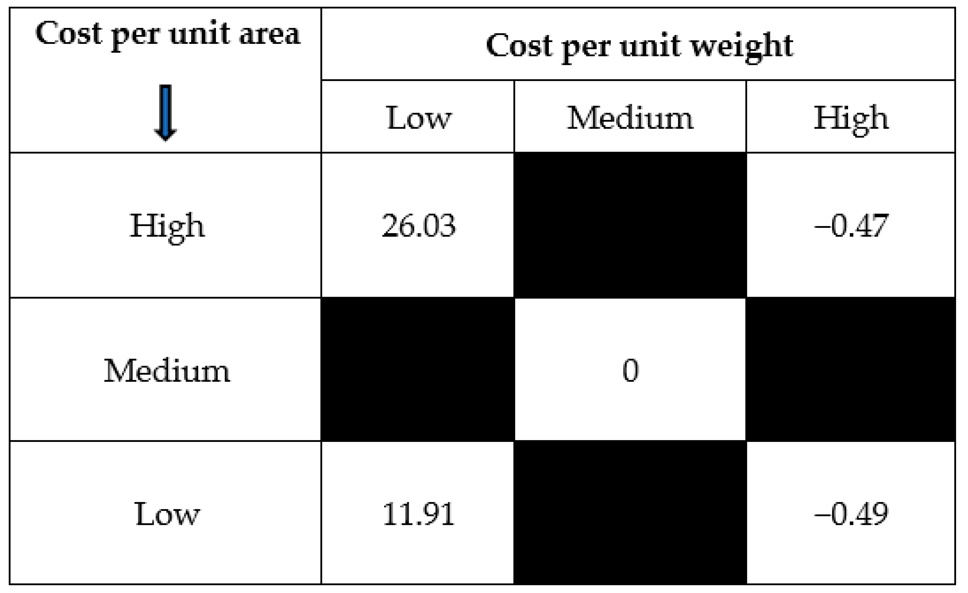
Organization-B is a trading organization with a large variety of products (more than 14,000 SKUs) used by dentists, which have a significant variation in the costs of items, price per unit weight, and price per unit volume. Therefore, the analysis was performed at the SKU level rather than a representative SKU from each product category. After validating the average inventory holding cost, the inventory holding cost for each SKU was sorted in ascending order; divided them into five groups, and picked the median value of block as shown in Figure 1. The variations in the calculated inventory holding costs for organizations A and B are provided in Figure 2 and Figure 3, respectively. The inventory holding cost of items that fall in the middle is the average cost of holding inventory. The rest of the values are the differences between the median value of that block and the average inventory. Therefore, negative values represent that an item’s inventory holding cost is less than the average cost of holding inventory. A positive value shows that it is higher than the average cost of holding inventory. It is important to mention that for Organization-B, the values in each cell are the median value, i.e., the extreme values in categories 1, 2, 4, and 5 are even larger (or smaller) than the values shown.
Implications of these findings will be discussed in the next section, along with a numerical example of the effects of these findings.
5. Numerical Example and Discussions
The numerical example below shows the effects of these findings in an organization dealing with various products and how it impacts an organization’s operational costs. The following data have been used:
| Demand rate (units/year) | D | 1000 |
| Production rate (units/year) | P | 3200 |
| Buyer’s order cost ($/order) | Kb | 25 |
| Vendor’s setup cost ($/batch) | Kv | 400 |
| Mean holding cost for the vendor ($ /unit/ unit of time) | hv | 4.00 |
| Mean holding cost for the buyer ($ /unit/ unit of time) | hb | 5.00 |
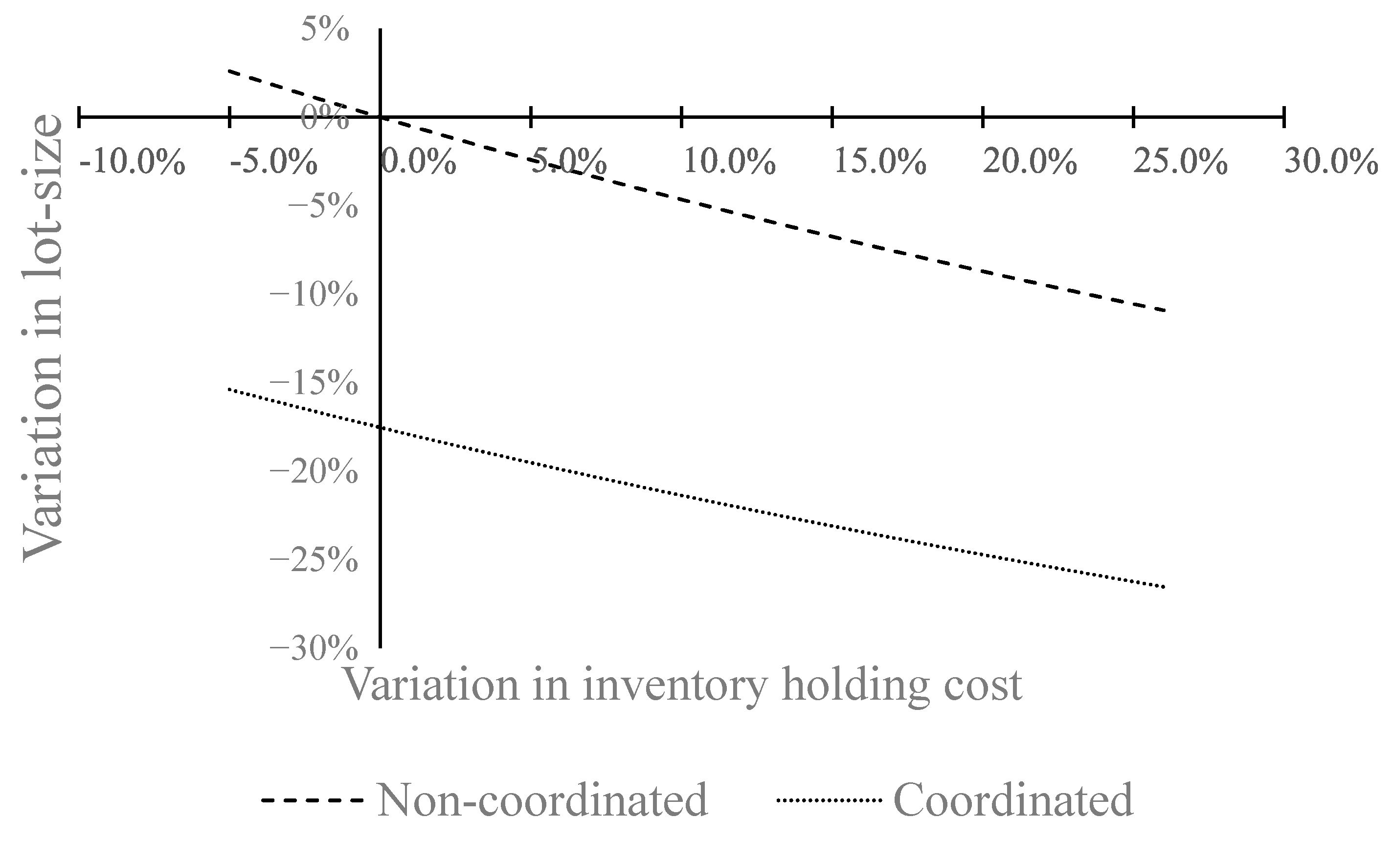
| Variation in inventory holding cost (%) | +25%/−0.5% |
Equation (10) provides the formula for classical EOQ (Harris 1913) and Equation (11) provides the formula for coordinated EOQ given by Banerjee (1986). The data has been taken from the paper of Gurtu et al. (2015a). The variations in lot size for a vendor and a buyer due to the changes in inventory holding costs are identical (Figure 4). The variations in inventory costs have been taken from the mean, and the range has been taken from the results of the analysis. As we know that the coordination provides a lower cost, the variations in the coordinated lot size are bigger than that of the non-coordinated lot sizes. The percentage changes in the lot size for buyer and vendor are identical.
The space cost-savings due to a reduction in lot size do not translate linearly in the overall inventory holding cost due to many other fixed costs of operation and maintenance. However, it translates to an overall savings of about 3%, keeping other parameters the same, and provides more storage space. For one of the organizations studied, this saving is about one hundred thousand. The savings are directional and will increase for a more expensive place.
It is interesting to see the clear difference in the inventory holding costs for these two organizations. The organization with a uniform input has a small variation in the inventory holding costs. On the other hand, inventory holding cost for items in a very diversified organization such as retail. The inventory carrying costs varies significantly as the products move away from the center in any direction in the grid (Figure 1). The cost of holding inventory is high for the products, which are lighter per unit value.
One of the takeaways of this analysis is that some products with a lower cost of holding inventory compensate for the products with a higher cost of holding inventory. The top management leaders assume that the cost of holding inventory is under control based on an average cost. However, finance department leaders need to evaluate inventory holding costs at the SKU levels to make an informed decision about using inventory holding costs at SKU levels or an average. SCM leaders need to pay attention to the items with a higher cost of holding inventory than the average inventory holding costs. These findings have minimal value for organizations with a single product or a family of products with very similar input costs per unit area. However, these findings are important for multi-product organizations such as retail for analyzing the inventory holding costs of each of their products or product categories. The order quantity calculated using the EOQ model with the new inventory holding cost will be different. In other words, this analysis for an organization will change the order quantity.
Further, this analysis suggests that there will be changes in the profit margin of a product or a product category due to the variations in the holding costs. In extreme cases, some products may have negative profit margins due to the high inventory holding cost. Finding a very high inventory holding cost for a product will lead to adjustments in the sourcing and sales policies. The changes in sourcing policies include inventory levels, finding a local vendor to reduce the lead time, changes in packaging, and storage at different locations. Changes in sales policies include changes in pricing, quantity discounts, and sales promotions, among others.
6. Conclusions
The purpose of this paper is to present a new way of calculating the cost of holding inventory for each item (SKU) in an organization instead of using an average cost of holding inventory. The paper analyzed the inventory holding cost for the various items in two organizations and found that using an average holding cost for all the items is not appropriate for organizations with a large variety of products that have variations in cost per unit weight and cost per unit area (or volume). The contributions of this paper are that (i) the inventory holding cost has significant variations for a multi-product organization, particularly in the retail industry, and (ii) inventory (and pricing) policies should be defined at the level of items (SKU) using the actual cost of holding inventory of individual items.
An average inventory holding cost has been used by academicians, practitioners, and advised by finance managers for over a century. The idea of using an average inventory is still valid for industries or organizations which have a single product or a small number of similar products, such as groceries, produce, dairy, apparel, to name a few. However, times have changed, and the business models have changed for many industries. As an example, the retail industry has transformed dramatically in the last five-six decades. Therefore, revisiting some of the established practices due to these changed circumstances is needed. This paper is a step in that direction. A retail organization or a big-box retailer has a large variety of products. Using an average cost of holding inventory is not appropriate for such organizations.
The analysis shows considerable variations in inventory holding cost due to the variations in cost per unit weight (weight-density) and cost per unit area or space (space-density) of products. Therefore, treating these costs as an average cost leads to selling some products with a higher profit margin and some at a very low-profit margin. Understandably, the profit margin of every product may not be the same in an organization. However, lower profit margins for a product should be by design rather than ignorance. It is also possible that due to this ignorance, some products are sold at a loss (negative profit margins) without acknowledging it. Therefore, the actual cost of holding inventory may lead to changing pricing and promotion policies for such products to minimize the loss.
This work has two limitations too. One of the limitations is that this concept has been tested on two organizations from two different industries, i.e., one organization from one industry. The second limitation is that the concept was validated in very close proximity, i.e., the variation found in the inventory holding cost within an industry may go up or down in different geographies. This leads to potential extensions of this work. Multiple organizations from the same industry from different geographies should be studied to see some inventory holding patterns. Another possible extension is to compare the variations in manual, semi-automatic, and automatic storage facilities. Another possible extension could be to study multiple warehouses of the same organization within a country to see the variation in the holding cost. Depending on the inventory holding cost, it may be possible to store different products in different locations. A study to optimize the total cost, including transportation cost, could be another possible extension.
Funding
This research received no external funding.
Informed Consent Statement
Informed consent was obtained from all subjects involved in the study.
Acknowledgments
Amulya Gurtu sincerely thanks the executives from (in alphabetical order) Dental City, Green Bay, WI, USA and Schreiber Foods, Green Bay, WI, USA for sharing their data for analyses.
Conflicts of Interest
The author declares no conflict of interest.
References
- Aljazzar, Salem M., and Amulya Gurtu. 2019. Observations on ‘a joint economic-lot-size model for purchaser and vendor’. International Journal of Inventory Research 5: 169–87. [Google Scholar] [CrossRef]
- Aljazzar, Salem M., Amulya Gurtu, and Mohamad Y. Jaber. 2018. Delay-in-payments—A strategy to reduce carbon emissions from supply chains. Journal of Cleaner Production 170: 636–44. [Google Scholar] [CrossRef]
- Arslan, M. Can, and Metin Turkay. 2013. EOQ Revisited with Sustainability Considerations. Foundations of Computing and Decision Sciences 38: 223–49. [Google Scholar] [CrossRef] [Green Version]
- Bahl, Harish C. 1982. A Noniterative Multiproduct Multiperiod Production Planning Method. Operations Research Letters 1: 219–21. [Google Scholar] [CrossRef]
- Balintfy, Joseph L. 1964. On a Basic Class of Multi-Item Inventory Problems. Management Science 10: 287–97. [Google Scholar] [CrossRef]
- Banerjee, Avijit. 1986. A Joint Economic-Lot-Size Model for Purchaser and Vendor. Decision Sciences 17: 292–311. [Google Scholar] [CrossRef]
- Battini, Daria, Alessandro Persona, and Fabio Sgarbossa. 2014. A sustainable EOQ model: Theoretical formulation and applications. International Journal of Production Economics 149: 145–53. [Google Scholar] [CrossRef]
- Braglia, Marcello, and Lucio Zavanella. 2010. Modelling an industrial strategy for inventory management in supply chains: The ‘Consignment Stock’ case. International Journal of Production Research 41: 3793–808. [Google Scholar] [CrossRef]
- Cárdenas-Barrón, Leopoldo Eduardo, Kun-Jen Chung, and Gerardo Treviño-Garza. 2014. Celebrating a century of the economic order quantity model. International Journal of Production Economics 155: 1–7. [Google Scholar] [CrossRef]
- Cárdenas-Barrón, Leopoldo Eduardo, Ali Akbar Shaikh, Sunil Tiwari, and Gerardo Treviño-Garza. 2020. An EOQ inventory model with nonlinear stock dependent holding cost, nonlinear stock dependent demand and trade credit. Computers & Industrial Engineering 139: 105557. [Google Scholar] [CrossRef]
- Chen, Wen, Qi Feng, and Sridhar Seshadri. 2015. Inventory-Based Dynamic Pricing with Costly Price Adjustment. Production and Operations Management 24: 732–49. [Google Scholar] [CrossRef]
- Chen, Xi, Saif Benjaafar, and Adel Elomri. 2013. The carbon-constrained EOQ. Operations Research Letters 41: 172–79. [Google Scholar] [CrossRef]
- Choi, Sangjin, and S. T. Enns. 2004. Multi-product capacity-constrained lot sizing with economic objectives. International Journal of Production Economics 91: 47–62. [Google Scholar] [CrossRef]
- Container Alliance. 2020. Shipping Container Specifications. Available online: https://www.containeralliance.com/specifications.php (accessed on 27 March 2020).
- CSI Containers Services International. 2020. ISO Container Size and Type (ISO 6346)—CSI Container Services International. Available online: https://www.csiu.co/resources-and-links/iso-container-size-and-type-iso-6346 (accessed on 27 January 2021).
- Dhandapani, J., and R. Uthayakumar. 2016. Multi-item EOQ model for fresh fruits with preservation technology investment, time-varying holding cost, variable deterioration and shortages. Journal of Control and Decision 4: 1–11. [Google Scholar] [CrossRef]
- Dobson, Gregory, Edieal J. Pinker, and Ozlem Yildiz. 2017. An EOQ model for perishable goods with age-dependent demand rate. European Journal of Operational Research 257: 84–88. [Google Scholar] [CrossRef]
- Eilon, Samuel. 1959. Economic Batch-Size Determination for Multi-Product Scheduling. Journal of the Operational Research Society 10: 217–27. [Google Scholar] [CrossRef]
- Ghasemkhani, A., R. Tavakkoli-Moghaddam, S. Shahnejat-Bushehri, S. Momen, and H. Tavakkoli-Moghaddam. 2019. An integrated production inventory routing problem for multi perishable products with fuzzy demands and time windows. IFAC-PapersOnLine 52: 523–28. [Google Scholar] [CrossRef]
- Goodarzian, Fariba, Hasan Hosseini-Nasab, Jesús Muñuzuri, and Mohammad-Bagher Fakhrzad. 2020. A multi-objective pharmaceutical supply chain network based on a robust fuzzy model: A comparison of meta-heuristics. Applied Soft Computing 92: 106331. [Google Scholar] [CrossRef]
- Goyal, S. K. 1977. An Integrated Inventory Model for a Single Product System. Operational Research Quarterly 28: 539–45. [Google Scholar] [CrossRef]
- Goyal, S. K. 1988. “A Joint Economic-Lot-Size Model for Purchaser and Vendor”: A Comment. Decision Sciences 19: 236–41. [Google Scholar] [CrossRef]
- Gurtu, Amulya, Mohamad Y. Jaber, and Cory Searcy. 2015a. Impact of fuel price and emissions on inventory policies. Applied Mathematical Modelling 39: 1202–16. [Google Scholar] [CrossRef]
- Gurtu, Amulya, Cory Searcy, and Mohamad Y. Jaber. 2015b. An analysis of keywords used in the literature on green supply chain management. Management Research Review 38: 166–94. [Google Scholar] [CrossRef]
- Gurtu, Amulya, Cory Searcy, and Mohamad Y. Jaber. 2017. Emissions from international transport in global supply chains. Management Research Review 40: 53–74. [Google Scholar] [CrossRef]
- Gurtu, Amulya, Cory Searcy, and Mohamad Y. Jaber. 2019. Transportation and Sustainable Supply Chain. In Handbook on the Sustainable Supply Chain. Edited by Joseph Sarkis. Northampton: Edward Elgar, pp. 410–28. [Google Scholar]
- Harris, Ford W. 1913. How Many Parts to Make at Once. Factory, The Magazine of Management 10: 135–136, 152. [Google Scholar] [CrossRef]
- Heinen, J. Jakob, and Kai Hoberg. 2019. Assessing the potential of additive manufacturing for the provision of spare parts. Journal of Operations Management 65: 810–26. [Google Scholar] [CrossRef] [Green Version]
- Jaber, Mohamad Y., and Saeed Zolfaghari. 2008. Quantitative Models for Centralized Supply Chain Coordination. In Supply Chain Theory and Applications. Edited by Vedran Kordic. Rejeka: InTech, pp. 307–38. [Google Scholar]
- Jaber, Mohamad Y., Simone Zanoni, and Lucio E. Zavanella. 2013. An entropic economic order quantity (EnEOQ) for items with imperfect quality. Applied Mathematical Modelling 37: 3982–92. [Google Scholar] [CrossRef]
- Khalilpourazari, Soheyl, and Seyed Hamid Reza Pasandideh. 2016. Multi-item EOQ model with nonlinear unit holding cost and partial backordering: moth-flame optimization algorithm. Journal of Industrial and Production Engineering 34: 42–51. [Google Scholar] [CrossRef]
- Khan, Mehmood, Mohamad Y. Jaber, and Abdul-Rahim Ahmad. 2014. An integrated supply chain model with errors in quality inspection and learning in production. Omega 42: 16–24. [Google Scholar] [CrossRef]
- Nagpal, Gaurav, and Udayan Chanda. 2021. Economic order quantity model for two generation consecutive technology products under permissible delay in payments. International Journal of Procurement Management 14: 93–125. [Google Scholar] [CrossRef]
- Pasandideh, Seyed Hamid Reza, Seyed Taghi Akhavan Niaki, and Behzad Maleki Vishkaei. 2014. A multiproduct EOQ model with inflation, discount, and permissible delay in payments under shortage and limited warehouse space. Production & Manufacturing Research 2: 641–57. [Google Scholar] [CrossRef]
- Perera, Sandun, Ganesh Janakiraman, and Shun-Chen Niu. 2017. Optimality of (s, S) policies in EOQ models with general cost structures. International Journal of Production Economics 187: 216–28. [Google Scholar] [CrossRef]
- Rajput, Neelanjana, R. K. Pandey, A. P. Singh, and Anand Chauhan. 2019. An optimization of fuzzy EOQ model in healthcare industries with three different demand pattern using signed distance technique. Mathematics in Engineering, Science and Aerospace 10: 205–18. [Google Scholar]
- Rastogi, Mohit, S. Singh, Prashant Kushwah, and Shilpy Tayal. 2017. An EOQ model with variable holding cost and partial backlogging under credit limit policy and cash discount. Uncertain Supply Chain Management 5: 27–42. [Google Scholar] [CrossRef]
- Santhi, G., and K. Karthikeyan. 2018. EOQ Pharmaceutical Inventory Model for Perishable Products with Pre and Post Discounted Selling Price and Time Dependent Cubic Demand. Research Journal of Pharmacy and Technology 11. [Google Scholar] [CrossRef]
- Sundara Rajan, R., and R. Uthayakumar. 2017. Analysis and optimization of an EOQ inventory model with promotional efforts and back ordering under delay in payments. Journal of Management Analytics 4: 159–81. [Google Scholar] [CrossRef]
- Tantiwattanakul, Phattarasaya, and Aussadavut Dumrongsiri. 2019. Supply chain coordination using wholesale prices with multiple products, multiple periods, and multiple retailers: Bi-level optimization approach. Computers & Industrial Engineering 131: 391–407. [Google Scholar] [CrossRef]
- Wahab, M. I. M., S. M. H. Mamun, and P. Ongkunaruk. 2011. EOQ models for a coordinated two-level international supply chain considering imperfect items and environmental impact. International Journal of Production Economics 134: 151–8. [Google Scholar] [CrossRef]
- Waters, Donald. 2003. Inventory Control and Management, 2nd ed. West Sussex: Wiley. [Google Scholar]
- Zahran, Siraj K., Mohamad Y. Jaber, Simone Zanoni, and Lucio E. Zavanella. 2015. Payment schemes for a two-level consignment stock supply chain system. Computers & Industrial Engineering 87: 491–505. [Google Scholar] [CrossRef]
- Zhang, Jiawei. 2009. Cost Allocation for Joint Replenishment Models. Operations Research 57: 146–56. [Google Scholar] [CrossRef] [Green Version]
- Zissis, Dimitris, George Ioannou, and Apostolos Burnetas. 2019. Coordinating Lot Sizing Decisions Under Bilateral Information Asymmetry. Production and Operations Management 29: 371–87. [Google Scholar] [CrossRef]
Figure 1.
Categorization of products.

Figure 2.
Variations in inventory holding costs of Organization A.

Figure 3.
Variations in inventory holding costs of Organization B.

Figure 4.
Variation in lot-sizes due to a change in holding cost.

Publisher’s Note: MDPI stays neutral with regard to jurisdictional claims in published maps and institutional affiliations. |
© 2021 by the author. Licensee MDPI, Basel, Switzerland. This article is an open access article distributed under the terms and conditions of the Creative Commons Attribution (CC BY) license (http://creativecommons.org/licenses/by/4.0/).
Share and Cite
MDPI and ACS Style
Gurtu, A. Optimization of Inventory Holding Cost Due to Price, Weight, and Volume of Items . J. Risk Financial Manag. 2021, 14, 65. https://doi.org/10.3390/jrfm14020065
AMA Style
Gurtu A. Optimization of Inventory Holding Cost Due to Price, Weight, and Volume of Items . Journal of Risk and Financial Management. 2021; 14(2):65. https://doi.org/10.3390/jrfm14020065
Chicago/Turabian StyleGurtu, Amulya. 2021. "Optimization of Inventory Holding Cost Due to Price, Weight, and Volume of Items " Journal of Risk and Financial Management 14, no. 2: 65. https://doi.org/10.3390/jrfm14020065