
Technique to Solve Linear Fractional Differential Equations Using B-Polynomials Bases


Department of Physics and Astronomy, University of Texas Rio Grande Valley, Edinburg, TX 78539, USA
*
Author to whom correspondence should be addressed.
Fractal Fract. 2021, 5(4), 208; https://doi.org/10.3390/fractalfract5040208
Submission received: 9 October 2021
/
Revised: 25 October 2021
/
Accepted: 2 November 2021
/
Published: 11 November 2021
(This article belongs to the Special Issue Frontiers in Fractional Schrödinger Equation)
Abstract
:A multidimensional, modified, fractional-order B-polys technique was implemented for finding solutions of linear fractional-order partial differential equations. To calculate the results of the linear Fractional Partial Differential Equations (FPDE), the sum of the product of fractional B-polys and the coefficients was employed. Moreover, minimization of error in the coefficients was found by employing the Galerkin method. Before the Galerkin method was applied, the linear FPDE was transformed into an operational matrix equation that was inverted to provide the values of the unknown coefficients in the approximate solution. A valid multidimensional solution was determined when an appropriate number of basis sets and fractional-order of B-polys were chosen. In addition, initial conditions were applied to the operational matrix to seek proper solutions in multidimensions. The technique was applied to four examples of linear FPDEs and the agreements between exact and approximate solutions were found to be excellent. The current technique can be expanded to find multidimensional fractional partial differential equations in other areas, such as physics and engineering fields.
1. Introduction
In real-world scientific phenomena, most problems follow either linearity or nonlinearity in their systems. In different fields, for example, engineering, computer science, and chemistry [1,2,3], fractional-order differential equations emerge more often. The most physical phenomena are described by the differential systems, which are integral-order systems. Many systems could be expressed with the help of the fractional differential equation [4,5,6,7,8,9]. Due to the materials and chemical properties of the real-world problems, and their memory and genetic characteristics, many physical problems follow fractional dynamical behavior [9,10,11]. The partial fractional-order differential equations are becoming a useful tool to model the physical phenomena [9]. For this reason, there has been an urgent need to find a solution to the fractional-order problems. However, there has been difficulty in obtaining the accurate analytical or numerical results of the most fractional-order differential model equations. There is a need for a suitable technique to find solutions to the fractional-order differential problems, linear and nonlinear. In our current paper, we aim to apply a technique to resolve multivariable linear fractional-order differential equations. Nonlinear fractional-order partial differential equations would be considered in future work. In recent years, many authors have used various numerical and analytical procedures to unravel fractional-order differential equations such as the modified simple equation approach [12,13,14,15] the variational iteration procedure [16], Adams–Bashfort–Mowlton Method [17], the Lagrange characteristic approach [18,19], Adomian decomposition method [20], the finite difference procedure [21], the differential transformation method [22], the finite element technique [23], the fractional sub equation procedure [24], the (/G)-expansion method [25], first integral approach [26], Jacobi–Gauss collocation method [27], the spectral collocation method (SCM) [28,29], and the fractional complex transform technique [30]. Every method has its own pros and cons.
In this study, we are going to implement the modified fractional-order Bhatti polynomial (B-poly) technique [31,32,33,34,35,36,37] that is significantly able to solve a variety of multivariable linear fractional-order differential equations. We chose the fractional-order B-poly due to its well-defined basis set and precision [33]. With these basis sets, it can be demonstrated that an arbitrary function can be represented to the desired accuracy and is directly differentiable over a closed interval. In several papers [31,32,33,34,35,36], using the B-poly basis of fractional-order and a generalized Galerkin method, the authors were able to find solutions to the fractional-order partial differential equations.
In an earlier work [31,32,33,34,35,36], the authors used a similar technique to find the solution to ordinary nonlinear and linear multidimensional differential equations. The current study focuses on linear fractional-order differential equations using the generalized Galerkin method [36] and the B-poly basis of fractional-order. This technique has the special advantage of the unitary partition property and the continuity of the generalized fractional-order B-polys over an interval [0, R], which are seamlessly differentiated. With the help of fractional-order B-polys, a fractional-order differential equation is transformed into an operational matrix using a matrix formalism that provides greater flexibility to the application of boundary as well as initial conditions on the operational matrix. The current study seeks solutions to four examples of linear fractional-order partial differential equations using the fractional-order B-poly technique. Employing Caputo’s fractional-order derivative definition, the derivatives of the fractional-order B-polys are taken. In the following sections, we present analytical formulism to employ Caputo’s fractional-order derivative on the polynomials, present the process used to create fractional-order basis sets, and develop an algorithm to resolve various linear fractional-order partial differential equations. We apply this technique to four examples. Finally, we shall present an error analysis of one of the fourth considered examples.
2. Caputo’s Fractional Differential-Order Operator
The explanation of the fractional-order derivative of Caputo is provided as [3]
where are Caputo’s fractional operator and fractional derivative in Caputo’s sense is , Equation (1). Caputo’s derivative of a constant is zero, i.e., and a fractional derivative of the polynomial is given by
Here, α denotes the order of the fractional function. The unknown two-variable dependent function is expanded as a product of two generalized fractional-order B-polynomials, , which may be considered as an approximate outcome to the FPD equation represented by
where is a j-th and m-degree fractional-order B-poly in variable with α as a fractional-order parameter over a given interval. The expansion coefficients in Equation (3) are the set of variables that are determined in the Galerkin scheme of minimization. Using Caputo’s derivative property as a linear operator, we can perform fractional differentiation
In the following section, we shall briefly mention the generalized fractional-order B-Polys basis, and some of their properties that could be useful to determine a solution of the linear fractional-order partial differential equation.
3. Fractional-Order B-Poly Basis
The generalized form of fractional B-polys in terms of variable x or t over an interval [0, R] or [0, T] are defined in Refs. [36,38]:
The fractional-order parameter α represents the fractional degree of the B-poly. There are (n + 1) fractional-order B-polynomials associated with any n value noted in Equation (5). The factor in Equation (5) is defined as
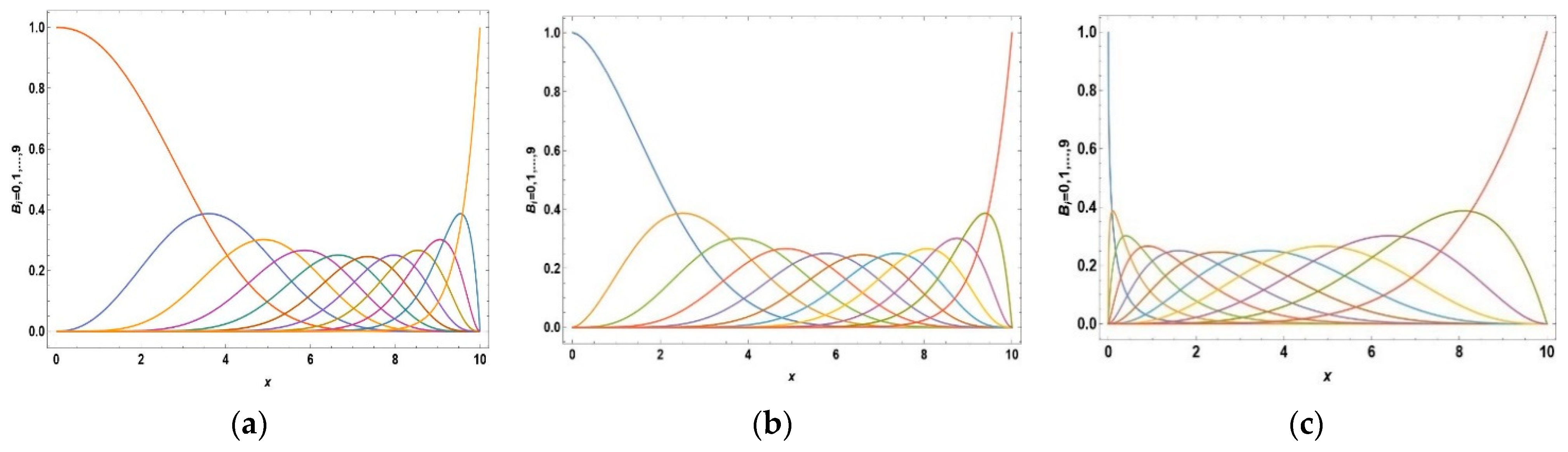
where this binomial coefficient is defined as, . For convenience, if i < 0 or i > n we can set . Mathematica or Maple software could be employed to develop all the non-zero fractional polynomials using a simple code prewritten with any value of n supported over an interval. The boundary conditions of the problem are generally associated with the first and last polynomial of the basis set. As an example, when n = 10 and fractional order are chosen in Equation (5), the corresponding basis sets of B-polys are plotted in Figure 1. Graphs of these fractional-order B-polys show how these B-polys add up to 1 at any given point, x. Such B-polys sets may be used to represent an arbitrary function with higher accuracy.
4. Technique for Approximating Solutions
Using the Galerkin method [36] and the generalized fractional-order B-poly basis set, we exploit a technique to seek practical solutions to fractional-order partial differential equations. We intend to apply Caputo’s fractional derivative to the fractional-order B-ploys. The examples of Caputo’s derivatives of the B-polys are provided in the last column of Table 1. Using the recent technique, we transform the fractional-order linear partial differential equation into an operational matrix and the initial conditions and boundary conditions are applied to the operational matrix. The presumed approximate solution, Equation (3) is substituted into the fractional-order differential equation and by-products are separated in terms of integral products in both variables x and t. Finally, both sides of the fractional equation are multiplied with fractional B-polys basis elements, , and the integrations are carried out using symbolic program, Mathematica, over the closed intervals [0, R] and [0, T], respectively. For example, the integration of the two fractional B-polys is given in the closed symbolic formula
Caputo’s derivative defined in Equation (2) is applied to the fractional B-ploy basis set, leading to the following closed results:
and the integrals of some arbitrary functions are given
With the help of these analytic formulas Equations (7)–(9), the operational matrix is constructed. The inverse of the operational matrix is required to find out the unknown coefficients of the linear combination in Equation (3). In the next section, we will describe our technique, as well as how to obtain a desirable result for the linear fractional-order partial differential equation. The technique will be employed in four examples to demonstrate that it works appropriately for approximating the accurate solutions. Plots of the approximate as well as exact solutions will be presented for comparison. An absolute error analysis of the fourth example will be introduced to show that, when the basis set of the fractional B-polys is enlarged, the accuracy of the solution is increased. Similarly, the error investigation can be carried out for other examples considered in this study. In the following section, for simplicity, we would like to drop off subscript and from the fractional B-polys, .
Example 1:
Let us introduce a linear partial fractional-order differential equation of the form
The ideal solution to Equation (10) is . A numerical solution is sought out in the intervals . The assumed solution, , is substituted into the Equation (10) and the result is presented below:
Caputo’s derivative operator is applied to Equation (11). The product of fractional B-polys from the basis set is multiplied on both sides of the Equation (11) and the integration on both variables is calculated over the intervals using a symbolic program. This operation provides the following equation
where with . The current technique leads to a system of equations. The elements of matrix are the unknown constants that are involved in those equations. After further simplification, the right-hand side column matrix and the matrix elements of operational matrix in terms of inner products of B-polys are given
The partial fractional-order differential Equation (10) is now transformed into a matrix equation . By deleting the rows and corresponding columns of the equation (13), the initial conditions are imposed on the operational matrix equation and the corresponding matrix W, so that the solution vanishes at t = 0 and x = 0. The operational matrix X was coded in the symbolic language Mathematica to determine its inverse. The inverse matrix was multiplied by the column matrix W to yield values of the unknown coefficients . The emerging estimated result is composed of the linear combination of the B-poly basis set via Equation (3). The process provides a valid approximate solution of the Equation (10) using B-polys of fractional-order and fractional differential-order of in Equation (10) is given below:
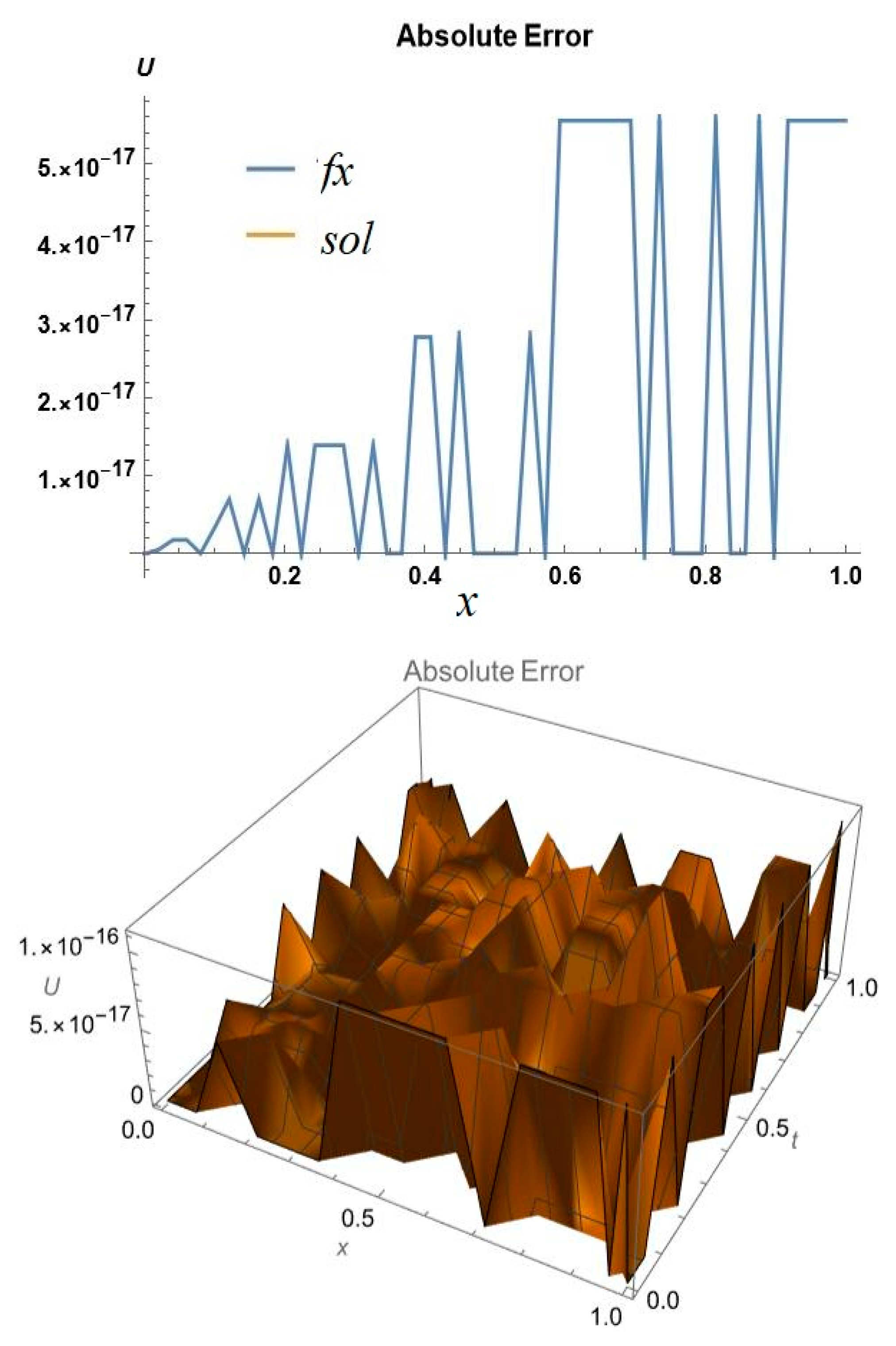
From the above result, it is noted that the approximate solution is very accurate. We have experimented with different values of fractional order of the differential equation while keeping the same order of the fractional polynomials basis set, the results remain the same with various values of . To solve the fractional-order partial differential Equation (10), we choose n = 1 and order B-poly basis set and in variables t and x, respectively. The corresponding coefficient values we obtained are . The Caputo’s derivative of the fractional B-poly basis set is , as seen in the last column of Table 1. A 3D plot of the estimated and the exact results of Equation (10) are presented in Figure 1 for comparison, and an excellent agreement can be seen between both results at the level of machine accuracy. Note that when t = x is substituted into Equation (14), the absolute error can be observed in the order of exhibiting the great aspect of constancy in one-dimension x. In the example, the absolute error between the results, both exact and approximate, shows that both results have excellent reliability. The absolute error in the 3D graph is also presented on the right-hand side in Figure 2. The 3D graph shows that the absolute error in the converged solution is of the order of .
Example 2:
Consider another example of fractional-order linear partial differential equation with different initial condition
The ideal solution of the Equation (15) is . The function , is called the Mittag–Leffler function [39] and is described as . In the summation of Mittag–Leffler function, we only kept k = 15 in the summation of terms. Therefore, the accuracy of the numerical solution will likely depend on the number of terms that we would keep in the summation of the Mittag–Leffler function. According to Equation (3), an estimated solution of Equation (15) using the initial condition may be assumed as After substituting this expression into the Equation (15). The Galerkin method, [29] and [32], is also applied to the presumed solution to obtain
Caputo’s fractional derivative is applied to Equation (16), and the product of fractional B-polys from the basis set is multiplied on both sides of the Equation (16). The resulting integration of both variables (t and x) is calculated over the intervals and , respectively. After further simplification of the Equation (16), we obtain
where the fractional-order derivative of the Mittag-Leffler function , with is used. The current technique leads to a system of equations. This system of equations may be summarized in the matrix equation , where the elements of matrix are the unknown constants. The right-hand side column matrix elements of and the matrix elements of operational matrix are given as
By deleting the rows and corresponding columns of Equation (18), the initial condition was imposed on the operational matrix, to make sure the solution vanishes at x = 0 and t = 0. The operational matrix X is inverted using Mathematica symbolic program and multiplied with the column matrix W to solve equation and yield values of the unknown coefficients . The emerging estimated result is composed of the B-poly basis set and the coefficients via Equation (3). The process provides an approximate solution to Equation (15) using B-polys of fractional-order and a fractional differential-order of . The final approximate solution is provided below:
To solve the fractional order partial differential Equation (15), we chose n = 15 and order B-poly basis set in both variables t and x. The corresponding fractional-order B-poly basis set is given in terms of variable x,
To obtain the B-polys basis set in variable t, we replace x = t. We have verified that as we enlarge the number of fractional-order B-polys set, the accuracy of the numerical solution increases. A 3D plot of the absolute error, between the estimated and exact solution of Equation (15), is presented for comparison in Figure 3, which presents the reliability between both results at the level of . Note that when is substituted in the solution Equation (19), the absolute error can be observed of the order of in one-dimension. The absolute error between the solutions, both approximate and exact, is found to be in good agreement.
Example 3:
Consider another partial fractional differential equation with an initial condition depending on the generalized fractional-order sine function
A numerical solution is pursued using the initial condition in intervals . The generalized definitions of sine and cosine function [3] are given
In this example, the assumed approximate solution contains an initial condition that has a generalized sine function as defined above. The efficiency of the numerical result is based on the number of terms that are kept in the summation of the generalized function. For this example, we kept k = 15 terms in the summation of the generalized sine function.
The exact solution of Equation (20) is . The approximated solution is substituted into the Equation (20) and the result is given below:
The Caputo’s derivative is applied to the above expression and the product of fractional B-polys from the basis, sets are multiplied on both sides of the Equation (21). The integration on both variables (x and t) is carried out over the intervals, respectively, and after further simplification, Equation (21) may be written in the form
The fractional-order derivative of the sine function is with . The technique leads to a system of operational matrix. This system of equations may be summarized in the matrix equation of the form , where the elements of matrix are the unknown constants. After further simplification, the right-hand side column matrix and the matrix elements of operational matrix in terms of inner products of B-polys are given as
To construct an appropriate solution to Equation (20), the partial fractional order differential Equation (20) is transformed into a matrix equation . By deleting rows and the corresponding columns of the Equation (23), the initial conditions are imposed on the operational matrix equation, so that the solution vanishes at t = 0 and x = 0. The operational matrix X is programmed in the symbolic language Mathematica to determine its inverse. The inverse of the matrix X is multiplied by the column matrix W and, by solving the matrix equation , the values of the unknown coefficients are determined. The resulting approximate solution is composed of the product of the B-poly basis set and the expansion coefficients, as in Equation (3). The technique provides the approximate solution to Equation (20) using 16 B-polys with n = 15, fractional-order and fractional differential-order of . The approximate solution is provided,
From the above result, it is noted that the desired approximate solution is converged and reached the desired accuracy. To find the solution to fractional-order partial differential Equation (20), we used the same fractional-order B-poly basis set as in Example 2. With the higher number (n) of fractional B-polys, a higher order of accuracy is achievable at the expense of computer CPU time. A 3D plot of the estimated and exact results of Equation (20) is presented in Figure 4 for the purpose of comparison. The plot shows an excellent agreement between both solutions at the level of . Note that when t = x is substituted in the Equation (24), the absolute error can be observed at the same level as exhibiting the great aspect of constancy in one-dimension x.
It is further noted that, from the traditional trigonometric identity, we know that
However, in Ref. [39] the authors state that, in fractional calculus, this kind of trigonometry identity does not hold. In this example, we have computationally proven that the above identity is no longer valid in fractional calculus, i.e.,
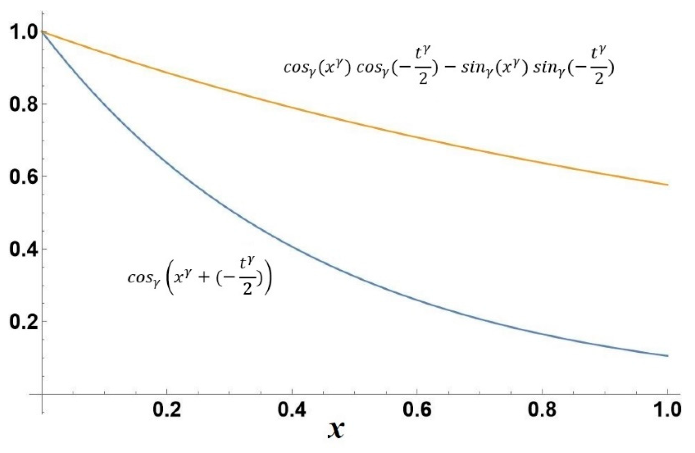
For further verification, we have plotted both sides of the identity Equation (26) and Figure 5 and they seem to disagree. For example, for , we show the graphs of both sides of the identity at x = t, (blue curve) and (yellow curve). From the graphs of both sides of the identity, we see that the blue and the yellow curves do not match. However, we know that when takes integral values, both curves overlap. We tried different and n values of B-polys; these curves still did not overlap. It is concluded that, in fractional calculus, certain traditional trigonometry identities may not be valid.
Example 4:
We consider a final example of the partial fractional-order differential equation with an initial condition as the generalized fractional-order cosine function,
A numerical solution is sought using initial condition [3], in the intervals . The assumed approximate solution contains an initial condition that has a generalized cosine function. The exact solution of Equation (27) is . The assumed solution, , is substituted into Equation (27) and the result is presented below:
After further simplification and applying the Caputo’s derivative, we obtain
where with . The current technique leads to a system of equations. This system of equations may be summarized in the matrix equation of the form , where the elements of matrix are the unknown constants. The matrix elements of the column matrix , and operational matrix are given as
The partial fractional-order differential Equation (27) is now converted into an operational matrix equation . By deleting the rows and corresponding columns of Equation (30), the initial condition is imposed on the operational matrix equation , so that the result has the correct behavior at t = 0 and x = 0. The inverse of matrix X is multiplied by the column matrix W to solve the matrix equation to yield the values of the unknown coefficients . The resulting approximate solution is composed of the product of the expansion coefficients and the B-poly basis set, as given in Equation (3). The technique provides the approximate solution of Equation (27) using n = 15 B-polys of fractional-order and fractional differential-order .
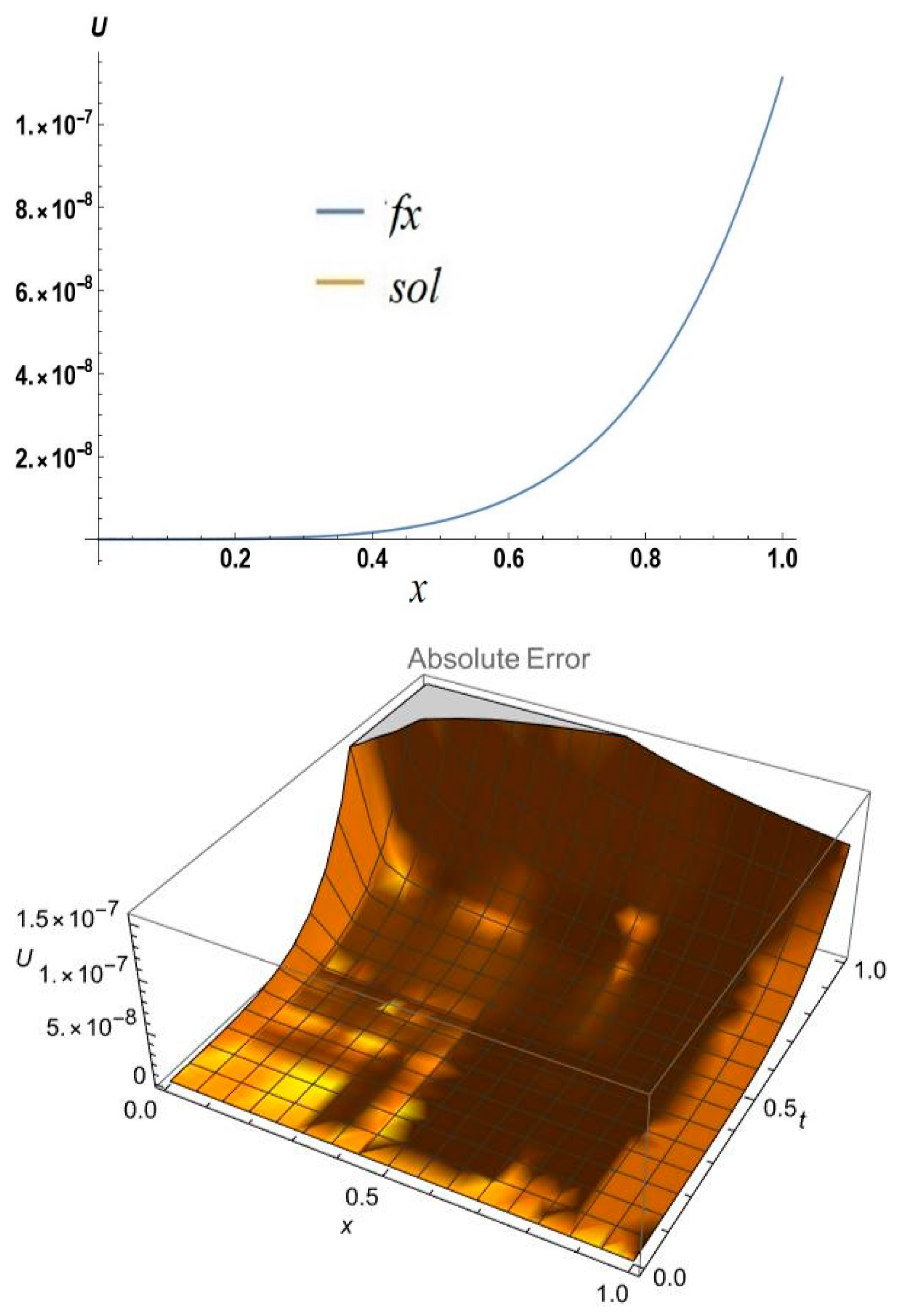
From the above result of Equation (31), it is noted that the approximate solution is converged and accurate. We have experimented with various values of fractional-order γ of the differential equation while keeping the same fractional-order polynomials basis set; the result remained the same at the desired level of accuracy. It is noted that when n = 6 set of B-polys is used, the absolute error is 10−3, and when n = 15 set of B-polys is used, the absolute error reduces to 10−7. It is concluded that with the increasing number of n sets of B-polys, a higher order of accuracy is attainable. In Table 2, we compare our calculated values with the exact values at various points for x and t. The absolute differences between the solutions are provided in the last column of Table 2, which shows excellent agreement. A 3D plot of the estimated and exact results of Equation (31) is presented in Figure 6 for the purpose of comparison. Note that when t = x is substituted in Equation (31), the absolute error in one dimension also goes to . The absolute error in the 3D graph is also presented in Figure 6 showing that the error in the converged solution is of the order of
From the traditional trigonometric rule, we know that the following is a valid identity
However, in Ref. [39], the authors state that, in fractional calculus, this trigonometry identity may not be true. In this example, we have computationally proven that the above identity is no longer valid in fractional calculus, i.e.,
For further verification, we have plotted both sides of the identity Equation (33) and they seem to disagree as shown in Figure 7. For example, for , we show the graphs of both sides of the identity at x = t, (blue curve) and (yellow curve). The graphs of both sides of the identity show that the blue and the yellow curves do not agree. However, we know that when takes integral values, both curves overlap. We tried different n values for B-polys and fractional values of , these curves still did not overlap. It is concluded that, in fractional calculus, this trigonometry identity may not be valid.
5. Error Analysis
We performed the calculations in the absence of a grid to solve linear fractional partial differential based on fractional B-polys. The fractional-order B-polys basis sets are defined on the intervals and . Our approximated results are dependent on the chosen (n) number of B-polys and the fractional-order modified Bhatti-polynomials. In this section, we present an error analysis based on the increasing number of B-poly basis sets; it is noted that the accuracy improves. The absolute error analysis for Example 4 is presented for the exact and approximate results. As you may have seen in Example 4, in the final calculation, we used the number k = 15 in the summation of the generalized formula for and also used n = 15 for the B-poly basis set in both x and t variables. Here, we want to show that as we set n = 6, the B-poly basis set would have only seven B-polys in it. We performed the calculations in Example 4; it is observed that the absolute error among solutions is of the order of 10−3. Next, we used n = 10, which would give us 11 B-poly sets. The absolute error among solutions reduces to the level of 10−6. Finally, we use n = 15, which would comprise 16 B-polys in the basis set. It is observed the error reduces to 10−7. We note that n = 15 leads to a 256 × 256-dimensional operational matrix, which is already a large matrix to invert. We had to increase the accuracy of the program to handle this matrix in the Mathematica symbolic program. Beyond these limits, it becomes problematic to find an accurate inversion of the matrix. Please note that increasing the number of terms in the summation (k-values in the initial conditions) also helps reduce error in the approximate solutions of the linear partial fractional differential equations. We can observe from the graphs (Figure 8 and Figure 9) that the absolute error decreases as we steadily increase the size of the fractional B-poly basis set. Due to the analytic nature of the fractional B-polys, all the calculations are carried out without a grid representation on the intervals of integration. We also presented the absolute error in terms of 3D graphs in Figure 2, Figure 3, Figure 4, Figure 5, Figure 6, Figure 7, Figure 8 and Figure 9. Clearly, the error is systematically decreased as the number of B-polys basis sets is increased in the calculations. The method provides a converged solution that is comparable with the exact solution. The CPU time for the calculation notably rises as we include a larger set of fractional B-polys in the computations.
6. Results and Discussions
In the current study, we investigated the 2D modified fractional Bhatti-polys basis set technique to determine the solutions to the partial fractional differential equations. Four examples of the linear partial fractional differential equations have been presented with various initial conditions and their semi-analytic solutions are also provided. Furthermore, an explanation of the 2D fractional algorithm process has been provided to calculate approximate solutions of the linear fractional differential equation. We estimated the results using the Galerkin method [40] in both variables (x, t). The graphs of the converged solutions are provided in Figure 2, Figure 3, Figure 4, Figure 5, Figure 6 and Figure 7. In the first example, the estimated solution was precise, which was equivalent to the exact solution after ignoring the tiny contributions. As the number of fractional B-polynomial basis set in the approximate solutions to Equation (3) was increased, the accuracy of the numerical solutions [36] increased. In our second, third, and fourth examples, we have used a value of n = 15 for the basis set of fractional B-polys in two variables (x, t). We also present 3D graphs of the precise and the approximated results of the absolute error in Figure 2, Figure 3, Figure 4, Figure 5, Figure 6, Figure 7, Figure 8 and Figure 9. In every case, the accuracy of the solutions was different because different B-poly basis sets and different operational matrix sizes were used. The numerical efficiency of the inverted matrix depends on the size of the matrix. In the last three examples, we used the series representation of the generalized sine and cosine functions; this requires the inclusion of many terms in the summation. When variable t was equal to x for 1D error analysis, the absolute errors among approximate and exact results were examined. The precision appears to be the same in both 1D and 3D error analyses. It is concluded that the present technique performed well in resolving linear fractional-order differential equations utilizing operational matrix scheme [40,41], as exhibited by the graphs and data shown in the study. We performed all integrations analytically and performed computations using Wolfram Mathematica symbolic program version-12 [42] for both x and t variables over the closed intervals.
The technique has presented great possibilities for solving linear multidimensional fractional differential equation problems in chemistry, physics, genetics, and other related disciplines. Nonlinear partial fractional differential equations will be investigated in another paper. Recently, many authors [43,44] have constructed operational matrices using B-polys methods to explain 1D partial differential equations. We have successfully expanded this technique to solve the 2D linear fractional differential equations. In our study, we also showed a detailed error investigation for the fourth problem that can be applied to other examples. The CPU time for computing the first example was less than 1 min, while examples 2–4 took 5–30 min of CPU time since those required a larger B-ploys basis set and higher dimensions of the operational matrix.
In this paper, we presented an expanded form of this technique [36] to determine solutions to linear partial fractional differential problems using fractional-order basis sets. This technique works well for resolving the equations connected to a complicated system of linear fractional-order differential problems where there are no known solutions. We may explore this method’s potential to solve 2D nonlinear partial fractional-order differential equations in forthcoming publications.
Author Contributions
Conceptualization, M.I.B.; software, M.I.B.; methodology, M.I.B.; formal analysis, M.I.B. and M.H.R.; validation, M.I.B., and M.H.R.; data curation, M.I.B. and M.H.R.; resources, M.I.B.; project administration, M.I.B.; investigation, M.I.B. and M.H.R.; supervision, M.I.B.; writing—original draft preparation, M.I.B.; writing—review and editing, M.I.B. and M.H.R. We confirm that the authors listed in the manuscript have been approved by all of us. All authors have read and agreed to the published version of the manuscript.
Funding
No external funding has been received for this research.
Institutional Review Board Statement
Not applicable.
Informed Consent Statement
Not applicable.
Data Availability Statement
The data that supports the findings are available within the article.
Acknowledgments
The authors would like to thank the Department for helping us to use the departmental computational facilities which have been utilized to execute the results of this study paper.
Conflicts of Interest
The authors declare no conflict of interest.
References
- Miller, K.S.; Ross, B. An Introduction to the Fractional Calculus and Fractional Differential Equations; John Wiley: Hoboken, NJ, USA, 1993. [Google Scholar]
- Kilbas, A.; Srivastava, H.M.; Trujillo, J.J. Theory and Applications of Fractional Differential Equations; North-Holland Mathematics Studies, 204, Fractional Calculus and Applied Analysis; Elsevier: Amsterdam, The Netherlands, 2006. [Google Scholar]
- Igor, P. An Introduction to Fractional Derivatives, Fractional Differential Equations, to Methods of Their Solution. In Fractional Differential Equations; Mathematics in Science and Engineering Series; Academic Press: Cambridge, MA, USA, 1998; Volume 198. [Google Scholar]
- Bagley, R.L.; Calico, R.A. Fractional order state equations for the control of viscoelasticallydamped structures. J. Guid. Control Dyn. 1991, 14, 304–311. [Google Scholar] [CrossRef]
- Sun, H.; Abdelwahab, A.; Onaral, B. Linear approximation of transfer function with a pole of fractional power. IEEE Trans. Autom. Control 1984, 29, 441–444. [Google Scholar] [CrossRef]
- Ichise, M.; Nagayanagi, Y.; Kojima, T. An analog simulation of non-integer order transfer functions for analysis of electrode processes. J. Electroanal. Chem. 1971, 33, 253–265. [Google Scholar] [CrossRef]
- Laskin, N. Fractional market dynamics. Phys. A Stat. Mech. Appl. 2000, 287, 482–492. [Google Scholar] [CrossRef]
- Kusnezov, D.; Bulgac, A.; Dang, G.D. Quantum Lévy Processes and Fractional Kinetics. Phys. Rev. Lett. 1999, 82, 1136–1139. [Google Scholar] [CrossRef] [Green Version]
- Li, C.; Zhang, F. A survey on the stability of fractional differential equations. Eur. Phys. J. Spec. Top. 2011, 193, 27–47. [Google Scholar] [CrossRef]
- Tavazoei, M.S.; Haeri, M. A note on the stability of fractional order systems. Math. Comput. Simul. 2009, 79, 1566–1576. [Google Scholar] [CrossRef]
- Torvik, P.J.; Bagley, R.L. On the Appearance of the Fractional Derivative in the Behavior of Real Materials. J. Appl. Mech. Trans. ASME 1984, 51, 294–298. [Google Scholar] [CrossRef]
- Jawad, A.J.M.; Petković, M.D.; Biswas, A. Modified simple equation method for nonlinear evolution equations. Appl. Math. Comput. 2010, 217, 869–877. [Google Scholar]
- Zayed, E.M.E. A note on the modified simple equation method applied to Sharma–Tasso–Olver equation. Appl. Math. Comput. 2011, 218, 3962–3964. [Google Scholar] [CrossRef]
- Wei, Y.; Guo, Y.; Li, Y. A new numerical method for solving semilinear fractional differential equation. J. Appl. Math. Comput. 2021, 1–23. [Google Scholar] [CrossRef]
- Mahor, T.C.; Mishra, R.; Jain, R. Analytical solutions of linear fractional partial differential equations using fractional Fourier transform. J. Comput. Appl. Math. 2021, 385, 113202. [Google Scholar] [CrossRef]
- Inc, M. The approximate and exact solutions of the space- and time-fractional Burgers equations with initial conditions by variational iteration method. J. Math. Anal. Appl. 2008, 345, 476–484. [Google Scholar] [CrossRef] [Green Version]
- Roman, P. Application of the Adams-Bashfort-Mowlton Method to the Numerical Study of Linear Fractional Oscillators Models. In AIP Conference Proceedings; AIP Publishing LLC.: Melville, NY, USA, 2021. [Google Scholar]
- Srivastava, H.M.; Alomari, A.-K.N.; Saad, K.M.; Hamanah, W.M. Some Dynamical Models Involving Fractional-Order Derivatives with the Mittag-Leffler Type Kernels and Their Applications Based upon the Legendre Spectral Collocation Method. Fractal Fract. 2021, 5, 131. [Google Scholar] [CrossRef]
- Guy, J. Lagrange characteristic method for solving a class of nonlinear partial differential equations of fractional order. Appl. Math. Lett. 2006, 19, 873–880. [Google Scholar] [CrossRef] [Green Version]
- Safari, M.; Ganji, D.D.; Moslemi, M. Application of He’s Variational Iteration Method and Adomian’s Decomposition Method to the Fractional KdV-Burgers-Kuramoto Equation. Comput. Math. Appl. 2009, 58, 2091–2097. [Google Scholar] [CrossRef] [Green Version]
- Cui, M. Compact finite difference method for the fractional diffusion equation. J. Comput. Phys. 2009, 228, 7792–7804. [Google Scholar] [CrossRef]
- Momani, S.; Odibat, Z.M. Fractional Green Function for Linear Time-Fractional Inhomogeneous Partial Differential Equations in Fluid Mechanics. J. Appl. Math. Comput. 2007, 24, 167. [Google Scholar] [CrossRef]
- Huang, Q.; Huang, G.; Zhan, H. A Finite Element Solution for the Fractional Advection-Dispersion Equation. Adv. Water Resour. 2008, 31, 1578–1589. [Google Scholar] [CrossRef]
- Guo, S.; Mei, L.; Li, Y.; Sun, Y. The Improved Fractional Sub-Equation Method and Its Applications to the Space-Time Fractional Differential Equations in Fluid Mechanics. Phys. Lett. Sect. A Gen. At. Solid State Phys. 2012, 376, 407–411. [Google Scholar] [CrossRef]
- Zheng, B. (G′/G)-Expansion Method for Solving Fractional Partial Differential Equations in the Theory of Mathematical Physics. Commun. Theor. Phys. 2012, 58, 623–630. [Google Scholar] [CrossRef]
- Lu, B. The first integral method for some time fractional differential equations. J. Math. Anal. Appl. 2012, 395, 684–693. [Google Scholar] [CrossRef] [Green Version]
- Peykrayegan, N.; Ghovatmand, M.; Skandari, M.H.N. On the convergence of Jacobi-Gauss collocation method for linear fractional delay differential equations. Math. Methods Appl. Sci. 2021, 44, 2237–2253. [Google Scholar] [CrossRef]
- Toh, Y.T.; Phang, C. Collocation Method for Fractional Differential Equation via Laguerre Polynomials with Eigenvalue Degree. In AIP Conference Proceedings; AIP Publishing LLC.: Melville, NY, USA, 2021. [Google Scholar]
- Khader, M.M.; Saad, K.M.; Baleanu, D.; Kumar, S. A spectral collocation method for fractional chemical clock reactions. Comput. Appl. Math. 2020, 39, 394. [Google Scholar] [CrossRef]
- Su, W.-H.; Yang, X.-J.; Jafari, H.; Baleanu, D. Fractional complex transform method for wave equations on Cantor sets within local fractional differential operator. Adv. Differ. Equ. 2013, 2013, 97. [Google Scholar] [CrossRef] [Green Version]
- Bhatti, M.I. Solution of Fractional Harmonic Oscillator in a Fractional B-poly Basis. Phys. Tech. Sci. 2014, 2, 8. [Google Scholar] [CrossRef]
- Bhatti, M.; Bracken, P.; Dimakis, N.; Herrera, A. Solution of mathematical model for gas solubility using fractional-order Bhatti polynomials. J. Phys. Commun. 2018, 2, 085013. [Google Scholar] [CrossRef]
- Bhatti, M.I. Analytic Matrix Elements of the Schrödinger Equation. Adv. Stud. Theor. Phys. 2013, 7, 11. [Google Scholar] [CrossRef]
- I Bhatti, M.; Hinojosa, E. 26 Results of hyperbolic partial differential equations in B-poly basis. J. Phys. Commun. 2020, 4, 095010. [Google Scholar] [CrossRef]
- Bhatti, M.I.; Rahman, H.; Dimakis, N. Approximate Solutions of Nonlinear Partial Differential Equations Using B-Polynomial Bases. Fractal Fract. 2021, 5, 106. [Google Scholar] [CrossRef]
- Bhatti, M.I.; Bracken, P. Solutions of differential equations in a Bernstein polynomial basis. J. Comput. Appl. Math. 2007, 205, 272–280. [Google Scholar] [CrossRef] [Green Version]
- Jong, S.-G.; Choe, H.-C.; Ri, Y.-D. A New Approach for an Analytical Solution for a System of Multi-term Linear Fractional Differential Equations. Iran. J. Sci. Technol. Trans. A Sci. 2021, 45, 955–996. [Google Scholar] [CrossRef]
- Bhatti, M.I. Solutions of the Harmonic Oscillator Equation in a B-Polynomial Basis. Adv. Stud. Theor. Phys. 2009, 3, 451–460. [Google Scholar]
- Massopust, P.R.; Zayed, A.I. On the Invalidity of Fourier Series Expansions of Fractional Order. Fract. Calc. Appl. Anal. 2015, 18, 1507–1517. [Google Scholar] [CrossRef] [Green Version]
- Fletcher, C.A.J. Computational Galerkin Methods; Springer: Berlin/Heidelberg, Germany, 1984. [Google Scholar]
- Alinhac, S. Hyperbolic Partial Differential Equations; Springer: Berlin/Heidelberg, Germany, 2009. [Google Scholar]
- Wolfram Research, Inc. Mathematica 12.0; Wolfram Research, Inc.: Champaign, IL, USA, 2019. [Google Scholar]
- Singh, A.K.; Singh, V.K.; Singh, O.P. The Bernstein Operational Matrix of Integration. Appl. Math. Sci. 2009, 3, 2427–2436. [Google Scholar]
- Farouki, R.T. Legendre–Bernstein basis transformations. J. Comput. Appl. Math. 2000, 119, 145–160. [Google Scholar] [CrossRef] [Green Version]
Figure 1.
(a) For n = 10, there is a total of 11 fractional B-polys of order . (b) For n = 10, there is a total of 11 fractional B-polys of order . (c) For n = 10, there is a total of 11 fractional B-polys of order . The graphs of the set of 11 B-polynomials are presented in the region x = [0, 10]. The , and are dimensionless quantities.

Figure 2.
A 1D plot of the absolute error between approximate (fx) and exact (sol) solutions is depicted on the left-hand for t = x changed in the solution, Equation (14). The 1D plot of the absolute error between approximate and exact results is also presented in the intervals and . The figure represents the consistency of the numerical solution is of the order of . This kind of accuracy occurred with only two fractional B-polynomials in the basis set.

Figure 3.
The absolute error plot between approximate (fx) and exact (sol) results is depicted on the left-hand side for t = x (1D plot). This graph is obtained when t = x is substituted in Equation (19). On the right-hand side, a 3D plot of the absolute error between exact and estimated solutions is also presented in the intervals and . Both graphs show that the efficiency of the numerical solutions is of the order of . This kind of accuracy was observed when n = 15 and order polynomial basis set was used.

Figure 4.
A 1D plot of the absolute error between approximate (fx) and exact (sol) solutions is presented on the left-hand side when t = x is replaced in Equation (24). The plot shows that the desired error is smaller. On the right-hand side, a 3D plot of the absolute error between approximate and exact results is also presented in the intervals and . The figure represents the efficacy of the numerical solutions is of the order of . This accuracy occurred with n = 15 number of fractional order B-poly basis set in x variable and the same basis set was used in t variable.


Figure 5.
Two graphs of the identity Equation (26) are presented to show that both sides of the identity do not agree for fractional values of . The left side of the identity is and the right side of the identity is at t = x. The values for and are used. The blue curve and the yellow curve do not agree or overlap. Hence, in general, the identity is invalid when fractional calculus is considered.

Figure 6.
A plot of the absolute error between approximate (fx) and exact (sol) solutions is introduced on the left-hand for t = x, Equation (31). The one-dimensional graph shows that the overlap of both results is pretty good. On the right-hand side, a 3D plot of the absolute error between approximate and exact results is also presented in the intervals and . The figure represents the effectiveness of the numerical solution is of the order of .

Figure 7.
Two graphs of the identity are presented to show that both sides of the identity do not match for fractional-order values of . The left side of the identity is and the right side of the identity is at t = x. The value for and are used. It is shown that the blue curve and the yellow curve do not agree. Hence, in general, the identity does not hold true when fractional calculus is considered.

Figure 8.
The absolute error between exact and approximate results of example 4 with n = 6 basis set of B-polys is presented in both variables (x, t), please see 3D graph. The estimated result is not converged. The values for are used.
Figure 8.
The absolute error between exact and approximate results of example 4 with n = 6 basis set of B-polys is presented in both variables (x, t), please see 3D graph. The estimated result is not converged. The values for are used.

Figure 9.
The absolute error analysis between exact and approximate results of Example 4 with n = 10 basis set of B-polys is presented in both variables (x, t), please see 3D graph. The estimated result is not converged. The values for are used.
Figure 9.
The absolute error analysis between exact and approximate results of Example 4 with n = 10 basis set of B-polys is presented in both variables (x, t), please see 3D graph. The estimated result is not converged. The values for are used.


Table 1.
For different values of (order of fractional-polynomials) and (order of the fractional differential equation), the table below shows fractional polynomial basis sets with n = 1, gives two B-polys and the corresponding derivatives. The symbol represents the Gamma function.
Table 1.
For different values of (order of fractional-polynomials) and (order of the fractional differential equation), the table below shows fractional polynomial basis sets with n = 1, gives two B-polys and the corresponding derivatives. The symbol represents the Gamma function.
| n | Basis Set | Caputo’s Derivative of Basis Set (Equation (2)) | ||
|---|---|---|---|---|
| 1/2 | 1/2 | 1 | ||
| 3/4 | 3/4 | 1 | ||
| 5/3 | 5/3 | 1 | ||
| 5/4 | 5/4 | 1 | ||
| 9/4 | 9/4 | 1 | ||
| 9/5 | 9/5 | 1 |
Table 2.
For different values of x and t, we compare our calculated approximated value with the exact value . We also provide their absolute difference.
Table 2.
For different values of x and t, we compare our calculated approximated value with the exact value . We also provide their absolute difference.
| x | t | Absolute Difference | ||
| 0.1 | 0.1 | 0.941097 | 0.941097 | 1.036 × 10⁻¹¹ |
| 0.2 | 0.2 | 0.886784 | 0.886784 | 1.091 × 10⁻¹⁰ |
| 0.3 | 0.3 | 0.836674 | 0.836674 | 5.120 × 10⁻¹⁰ |
| 0.4 | 0.4 | 0.790420 | 0.790420 | 1.660 × 10⁻⁹ |
| 0.5 | 0.5 | 0.747668 | 0.747668 | 4.333 × 10⁻⁹ |
| 0.6 | 0.6 | 0.708152 | 0.708152 | 9.785 × 10⁻⁹ |
| 0.7 | 0.7 | 0.671593 | 0.671593 | 1.991 × 10⁻⁸ |
| 0.8 | 0.8 | 0.637742 | 0.637742 | 3.744 × 10⁻⁸ |
| 0.9 | 0.9 | 0.606376 | 0.606376 | 6.617 × 10⁻⁸ |
| 1.0 | 1.0 | 0.577288 | 0.577288 | 1.112 × 10⁻⁷ |
Publisher’s Note: MDPI stays neutral with regard to jurisdictional claims in published maps and institutional affiliations. |
© 2021 by the authors. Licensee MDPI, Basel, Switzerland. This article is an open access article distributed under the terms and conditions of the Creative Commons Attribution (CC BY) license (https://creativecommons.org/licenses/by/4.0/).
Share and Cite
MDPI and ACS Style
Bhatti, M.I.; Rahman, M.H. Technique to Solve Linear Fractional Differential Equations Using B-Polynomials Bases. Fractal Fract. 2021, 5, 208. https://doi.org/10.3390/fractalfract5040208
AMA Style
Bhatti MI, Rahman MH. Technique to Solve Linear Fractional Differential Equations Using B-Polynomials Bases. Fractal and Fractional. 2021; 5(4):208. https://doi.org/10.3390/fractalfract5040208
Chicago/Turabian StyleBhatti, Muhammad I., and Md. Habibur Rahman. 2021. "Technique to Solve Linear Fractional Differential Equations Using B-Polynomials Bases" Fractal and Fractional 5, no. 4: 208. https://doi.org/10.3390/fractalfract5040208