Wind Farm Yaw Optimization via Random Search Algorithm

1
Department of Mechanical Engineering, California State University, Los Angeles, CA 90032, USA
2
School of Aeronautics, Northwestern Polytechnical University, Xian 710072, China
*
Author to whom correspondence should be addressed.
Energies 2020, 13(4), 865; https://doi.org/10.3390/en13040865
Submission received: 9 December 2019
/
Revised: 6 February 2020
/
Accepted: 11 February 2020
/
Published: 16 February 2020
(This article belongs to the Special Issue State of the Art of Wind Farm Optimization)
Abstract
:One direction in optimizing wind farm production is reducing wake interactions from upstream turbines. This can be done by optimizing turbine layout as well as optimizing turbine yaw and pitch angles. In particular, wake steering by optimizing yaw angles of wind turbines in farms has received significant attention in recent years. One of the challenges in yaw optimization is developing fast optimization algorithms which can find good solutions in real-time. In this work, we developed a random search algorithm to optimize yaw angles. Optimization was performed on a layout of 39 turbines in a 2 km by 2 km domain. Algorithm specific parameters were tuned for highest solution quality and lowest computational cost. Testing showed that this algorithm can find near-optimal (<1% of best known solutions) solutions consistently over multiple runs, and that quality solutions can be found under 200 iterations. Empirical results show that as wind farm density increases, the potential for yaw optimization increases significantly, and that quality solutions are likely to be plentiful and not unique.
1. Introduction
Wind turbine wakes are undesirable as they reduce energy production and increase mechanical stresses of downstream turbines. These wake interactions can reduce annual energy production up to 10% to 20% [1]. As wind passes through a wind turbine it creates a wake that detrimentally affects the power generated by turbines downstream. One way to reduce wake effect during planning stage is place wind turbines strategically within a domain, and this has been well studied [2,3,4,5,6,7,8,9,10,11,12,13,14,15,16,17,18,19,20,21]. Many of these studies focused on developing novel optimization algorithms to minimize wake effects. Other studies focused on developing optimization models and algorithms to solve multi-objective functions beyond purely minimizing wake effects, such cost, cabling, land constraints, noise.
In addition to optimizing turbine locations, yaw optimization and control of individual turbines can also reduce wake loss and improve the power production [22,23,24,25,26,27,28,29,30,31,32]. By yawing upstream turbines, wakes can be deflected away from downstream turbines. In particular, several studies [28,29,31,32] were conducted to study the potential improvement of controlling turbine yaw angles. Fleming et al. [24] performed an numerical analysis on two turbines and concluded that the overall power production could be increased with optimized yaw angles. There are some existing work in yaw angle optimization [25,28,32] which demonstrated that yawing optimization can reduce wake losses significantly, and that optimizing yaw angles based on wind direction is more important than optimizing to wind speed. Although yawed turbines will produce less energy, the downstream wakes are deflected away from turbines downstream, leading to an overall increase in energy production. However, optimizing yaw angles within a farm is an non-trivial task, as there are infinite combinations of yaw angles in every wind farm.
The aim of wind farm yaw control and optimization is to maximize power production by minimizing wake interactions. One approach is to accurately describe the complex physical interactions within the wind farm, and directly develop control strategies based on this description [23,27,32,33]. However, due to the complexity of turbulent atmospheric flow, the computational cost required to accurately simulate all the conditions is immense, thus real-time wind farm power optimization using high-fidelity flow simulations is not yet possible [29,34].
In recent years, low cost wake models capable of simulating yawed wakes which are suitable for fast yaw optimization have been developed. Jiménez et al. [23] derived a simple wake deflection model of turbines in yaw, but subsequent studies [35,36,37] demonstrated that the model tends to overestimate wake deflection. Bastankhah and Porté-Agel [26] developed a computationally inexpensive analytical wake model to predict wake deflection and velocity distribution in the far wake; however, this model does not adequately account for turbulence intensity, which is important in wake development. Qian and Ishihara [35] developed a mechanistic analytical wake model accounting for turbulence intensity, and validated with experimental results. Then, Lopez et al. [38] developed an accurate and low-cost numerical field model, building on the unyawed wake model by Kuo et al. [39] and the yawed wake model by Qian and Ishihara [35]. Shapiro et al. [40] derived a new model based on the aerodynamic lifting line theory.
In conjunction with these wake models and wind farm data, control algorithms can be used to optimize yaw angles. Several studies have developed optimization-based control approaches to adjust to the uncertainties, using approaches such as Bayesian optimization [41], genetic algorithm [42], game theory [43,44], random search [45], sequential optimization [32], gradient descent [28,46], greedy control [47], particle swarm optimization [48], dynamic programming [49,50]. Most recently, Howland et al. [37] developed an control scheme based on an empirical fitted analytical wake model [26,40]. This analytical wake model was calibrated for a six turbine group within a wind farm in Alberta, Canada based on historical data. Then wake steering is done by solving a yaw optimization model in real-time using a gradient descent strategy called Adam optimization [51]. Over the period tested, the wind farm production increased by 7–13% near average wind speeds and decreased production variability by up to 72%.
To solve the optimization problem in real-time, particularly for higher number of turbines, it is important to reduce computational cost. A number of optimization algorithms have been developed to optimize wind farm layout [6,16,52,53,54,55]. Keeping in mind of the lessons learned from layout optimization literature, the objective of this work is to develop an optimization algorithm to optimize yaw angles of a wind farm, with emphasis on solution quality and low computational cost. In this work, we propose a random search (RS) algorithm, and we apply this algorithm in conjunction with a steady analytical wake model by Qian and Ishihara [35] to compare its performance with that of a binary quadratic programming model, in terms computational cost and solution quality. The remainder of the paper is structured as follows: Section 2 focuses on the wake model used in this work; Section 3 discusses the proposed RS algorithm and the model to be solved; Section 4 illustrates and discusses the performance of the algorithm; and Section 5 summarizes the findings.
2. Wake Model
This work is utilizes the wake model by Qian and Ishihara [35] with the proposed optimization algorithm. This yaw wake model states the relationship between the average wake velocity, , and velocity deficit, , and is described as
where, is the freestream velocity of the wind.
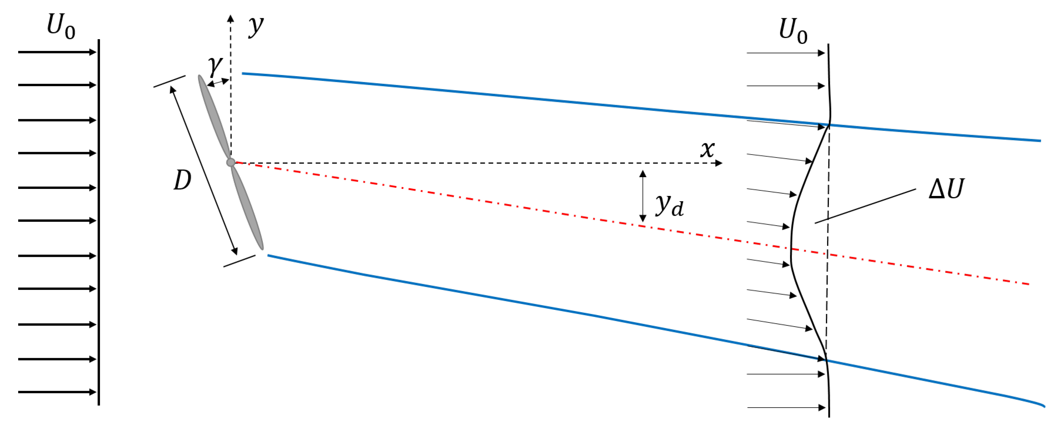
As shown in Figure 1, is related to both x (i.e., the distance measured downstream from the turbine) and (i.e., radial distance measured from the center of the yawed wake) in plane, and can be found by using
where S in Equation (2) is the streamwise function, and can be found by using,
Here, represents the yaw angle, D represents the diameter of turbine (illustrated in Figure 1), is the ambient turbulence intensity, and is the coefficient of thrust under no yawing conditions. In this form, Equation (3) is applicable in the far wake region.
To capture the change in velocity deficit (Equation (2)) in the spanwise direction, a spanwise function is used, and this is described using a Guassian function,
Here, is the standard deviation of the wind velocity distribution at each cross-section, and can be calculated through
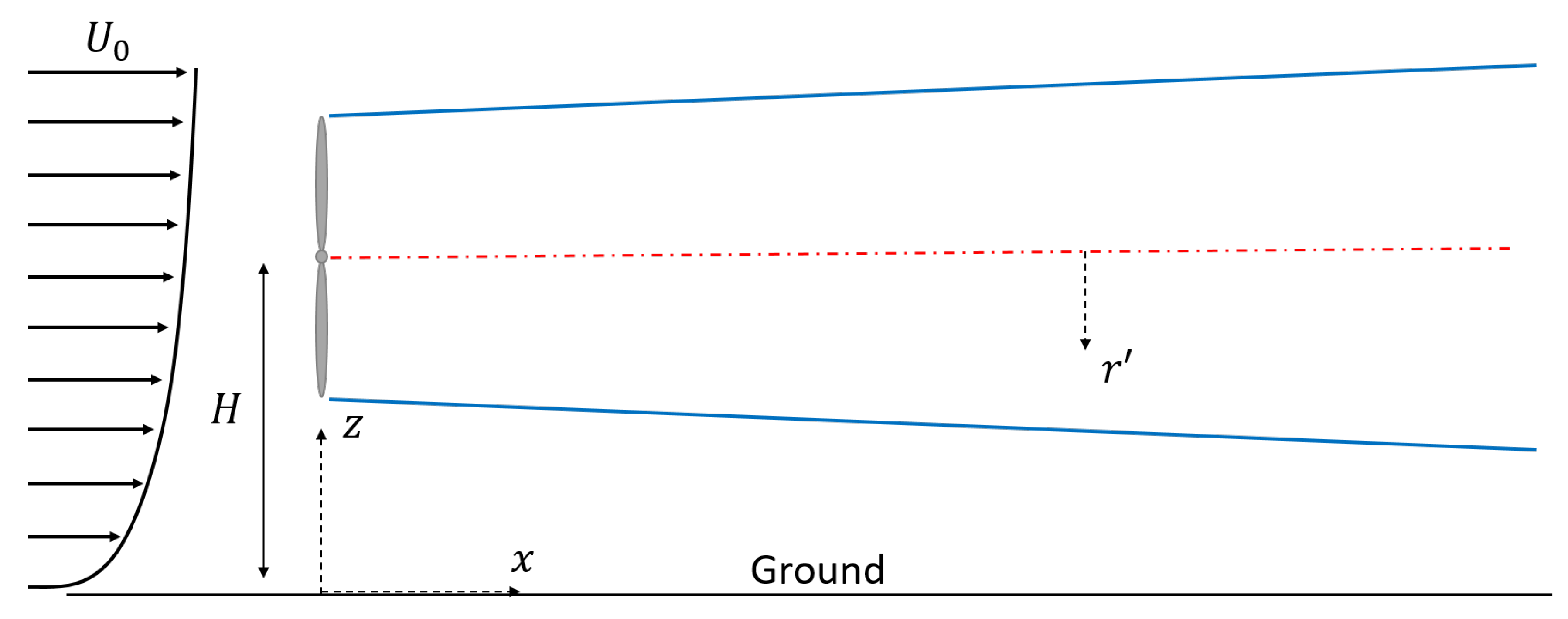
where in Equation (4) is the radial distance measured from the center of the yawed wake in plane, as illustrated in Figure 2, and can be defined by
Here, H is the hub height; is the wake deflection, and its expression depends on its location within the wake. In the near wake region, is assumed to be linear with distance downstream of turbine and is expressed as
and,
where is the initial skew angle. In the far wake region, is expressed as
where is the wake deflection and is the standard deviation of the velocity distribution at the end of near wake region, , and
and
This analytical model can only be used to calculate the downstream velocity caused by a single yawed turbine. If a wake of ith
turbine is influenced by n multiple nearby upstream yawed turbines, the downstream velocity, , needs to be calculated through
where, represents the wind velocity at ith turbine due to the wake of jth turbine. If the turbine is partially immersed in an upstream turbine wake, then is the rotor area immersed in the upstream wake. Details on can be found in the work by González et al. [56].
3. Optimization Formulation and Random Search Algorithm
3.1. Optimization Formulation
The objective of the optimization problem is to maximize power production of a wind farm. The problem formulation for the optimization problem is as follows:
where the number of turbines in a wind farm is N and n is the number of turbines upstream of turbine i. A single wake model is used to solve for the velocity at turbine i due to the wake of turbine j, denoted as . In this formulation, each turbine i is allowed to yaw freely, at angle . Furthermore, is density of air, A is rotor area of turbine, and is the power coefficient of the turbine i. The power curve of a turbine is dependent on the model and manufacturer, but an ideal curve is used in this study, and we assume that the coefficient of power of a yawed turbine is proportional to cosine of yaw angle squared, similar to empirically observations [25,57,58]. That is, at an yaw angle of . Note that there is no physical explanation behind this cosine dependence other than it created a good fit with experimental results.
3.2. Proposed Random Search Algorithm
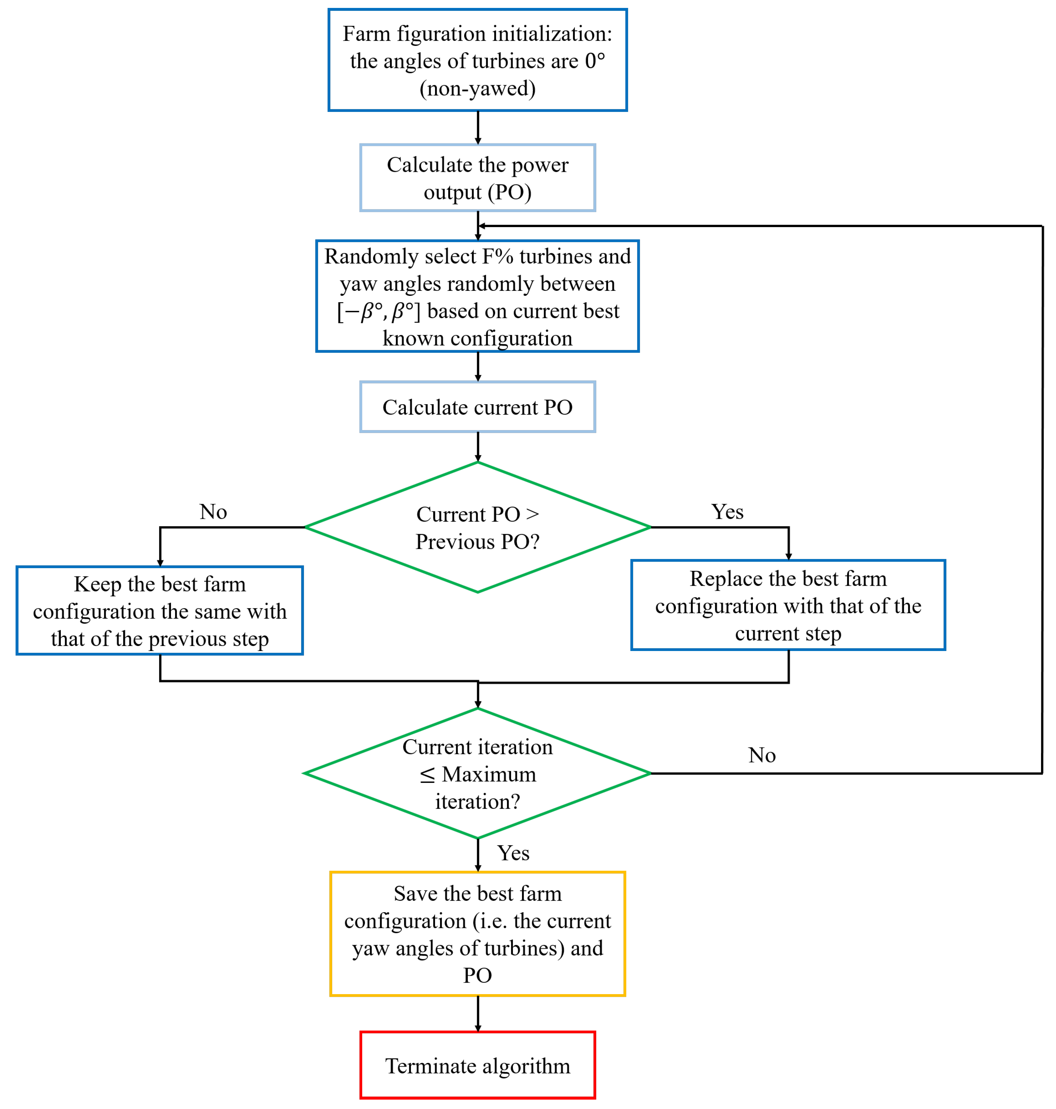
The authors initially developed an BQP model [59], which allows turbines to yaw a predefined set of angles. The authors’ experience developing and working with mathematical programming models for wind farm layout optimization problems suggested that this BQP model can be quickly solved using state-of-the-art solvers such as Gurobi and CPLEX, and perhaps outperform certain types of metaheuristic algorithms. However, it became clear that the BQP model is not suitable for fast optimization purposes as the size of the problem grows exponentially with increasing size of the set of angles. From our experience developing the BQP model and analyzing results, we realized that near-optimal (<1% of best known solutions) solutions are plentiful and that systematically guessing solutions is likely to do well. This leads to the proposed RS algorithm.
The core idea behind the proposed algorithm is to improve solution quality based on best known solution during the optimization process. Thus, instead of determining the yaw angle, , the algorithm determines an incremental yaw angle with respect to the current yaw angle. This incremental yaw angle is randomly selected from a range of to , where the value of is predefined. As shown in Figure 3, the algorithm starts with the determination of the power output of a farm with all non-yawed turbines, which is considered as the initial farm configuration. This initial configuration is considered to be the best known configuration. Then, the yaw configuration of the farm is changed by yawing of the turbines to angles ranging from to . After that, the power output of the farm with new configuration is calculated and compared to that of the best configuration. If the new configuration produces higher power production, then the best known configuration will be replaced by the new configuration. Based on the best known solution, the turbines will yaw additionally and randomly between the range of and and compared with the previous solution. This process is repeated for a specified number of iterations. In other words, the yaw angle of a turbine i, , will be the sum of all the random angles chosen between and from previous iterations. For example, suppose , and turbine 1 yaws (random selected between to ) from the initial yaw angle of relative to the wind in the first iteration, then yaws (random selected between to ) from its current yaw angle in the second iteration, so the yaw angle of the turbine after two iterations is , if both configurations produced higher larger power output than previous configurations.
This simple algorithm builds upon best known solutions to find the better solutions. To reduce the computational cost and improve the quality of solutions, determination of the percentage of turbines to be yawed, F, and the range of angle are crucial to achieve those objectives. For instance, if is large, there is a strong likelihood to find very different solutions than the initial baseline solution. Conversely, if is small, it is likely that the new solution will be similar to the initial baseline solution. Thus, the value of can be seen as a mean to control intensification and diversification of the optimization process. The percentage of turbines yawed in a single iteration, F, is important as well in terms of solution quality and computational cost. If F is a small value, the change per iteration will be small and may likely slow down convergence and further increase computational cost. If the value of F is large, the additional computational cost associated with each mathematical operation may not become negligible, but there is no guarantee that the solution quality will increase, especially during the intensification process. The detailed explanation of choice of F and is illustrated in the Section 4.
The termination criteria in the proposed algorithm is dependent on the number of iterations. Of course, more complex convergence criteria could be implemented; however, since computational cost is of importance in real-time yaw control, constraining the computational cost by fixing the maximum number of iterations is also applicable. Clearly, as the value of maximum iteration increases, better solutions will always be found, thus we are interested in determining the best possible solutions within a realistic time frame. The value of maximum iteration was set to be 1000 iterations.
4. Results
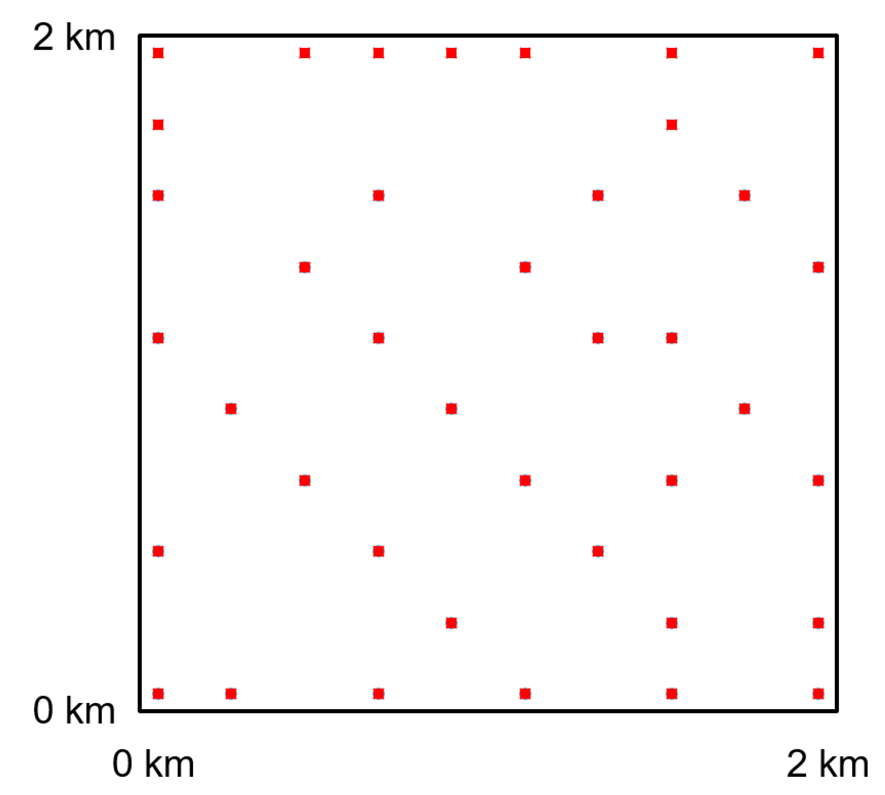
The optimal wind farm layout used in this work is from Grady et al., shown in Figure 4. This optimized layout is based on a wind speed of 12 m/s uniformly from 36 different wind direction sectors separated by , and each wind direction sector is a 10 degree wind sector. For example, wind direction sector is a wind sector ranging from to . The diameter of the 39 turbines is m, hub height of 60 m, and . These parameters are shown in Table 1. The optimal layout from this simple wind regime shows turbines evenly spread out throughout the domain and that there are no turbine clusters. We will be performing yaw optimization on this layout to study the performance of the RS algorithm.
It is important to note that in this study, we only consider fixed values for and . However, under experimental condition, these parameters are functions of tip speed ratio and yaw angle. Thus, these simplified assumptions would lead to errors in predicting power production. Nevertheless, as this work is focused on studying the performance of optimization approaches, these simplifications are justified as they are commonly used in the literature.
The algorithm in this paper was implemented in MATLAB (i.e., MATLAB 2019) and solved using an HP EliteDesk with a 4 core Intel i5-6500 3.2 GHz processor and 8 GB of RAM. To ensure a high quality of optimal solution and low computational cost, the maximum number of iterations is set to be 1000. Under current MATLAB implementation, it takes approximately 3 s per iteration on the 4-core desktop. It is clear that even at 1000 iterations, the computational cost for RS algorithm is significantly lower than the 16 CPU hours used to solve the BQP model. The optimization problem is solved for each wind direction at degree increment, and then averaged over their corresponding sector, for all 36 different wind direction sectors. The results of this work is compared to that of BQP model, discussed in the following subsections.
4.1. Identifying
To investigate the effects of range of incremental yaw angle, , and their effect on optimality and computational cost, the following angle ranges are considered, , , , and , or . As mentioned in Section 3, larger values of (e.g., and ) should be used if we wish to explore the search space (diversification) and the smaller values of (e.g., and ) if we wish to concentrate on promising regions (intensification). During the diversification process, the focus is to find a number of good solutions earlier in the optimization process. Then, later in the process, an intensification process would take place to refine solution quality. Thus, it may not be ideal to consider a single value throughout the the optimization process.
Thus, we consider a decaying function for , which varies the value of during the optimization process to balance between solution quality and computational time, and the results are compared with fixed values. The idea of this decaying function is similar in concept to the probabilistic function in simulated annealing [61]. The value of should be larger early on in the optimization process to take risks and explore different neighborhoods, and gradually decrease with increasing number of iterations. Then, we define as , where k is an exponential constant to be determined and g is the number of iteration, and has an asymptote of . Note that this equation was developed with an termination point of 1000 iterations (hence the exponent ), and that this should be modified for different maximum iteration. Here we consider the value of m to be 4, and k to be 5 and 8. We compare the results with the decay function with constant values, shown in Table 2, which shows the percent improvement in power (solution quality) after 1000 iterations over five trials, with the top five objective values underlined. It can be seen that in terms of solution quality, the results using the decay function are similar to that of fixed values. Three important observations can be drawn from these experiments. First, most trials reach nearly identical objective values. There are likely numerous local optima with similar objective values, and that all approaches will eventually find one. Second, when value is small, e.g., , the number of iterations it takes to find near-optimal (<1% of best known solutions) solution increases. As the value increases to , the number of iterations required to find near-optimal solution decreases. However, when the value of increases to and , although good solutions are found early on, solution quality improvement becomes stagnant later in the optimization process. Third, all values tried with the exception of all resulted in similar performance, ranging between 6.3% to 6.5%. This means that the algorithm is robust in finding good solutions and that diversification is likely to be more important than intensification in this type of problem.
4.2. Identifying F
Identifying the percentage of turbines, F, to be yawed in each iteration is important. It is worth noting that as the value of F increases, the ability to fine tune solutions decreases as more randomness is present in each iteration, especially later on in the optimization process. The value of F is varied to study how it affects solution quality and computational cost. We performed five trials for 13 different values of F, corresponding to different number of turbines which will be yawed in each iteration. These trials were performed with a decay function constants of and . As previously mentioned in Section 3, when the value of F is small, it would take many iterations to find good solutions as it searches through the search space at a slower pace. When the value of F is very large, randomness will dominate as a single turbine could be yawed multiple times within a single iteration, thus producing similar effects as increasing the range of . Table 3 shows the average solution (of five trials) found at the end of 100, 200, 300, 500, and 1000 iterations. The values are shown in terms of percentage increase from unyawed solution, averaged over five trials. The best solutions after 50 iterations are found with F values in the range of 17.9% and 51.3%. After 200 to 300 iterations, the best range of F lies between 7.7% to 51.3%. However, after 500 iterations, the best F values reduces to a range of 7.7% to 25.6%. After 1000 iterations, the ideal range lies between 5.1% to 25.6%. In other words, higher F value emphasizes on exploring the search space, and will produce better solutions earlier on in the search, while lower F value intensifies the search, which finds better solutions later on in the optimization process. However, after 1000 iterations, the quality of solutions found for all F values tested, with the exception of and , resulted in greater than increase in performance, illustrating the robustness of the algorithm. For the remainder of this work, the values , , and are used.
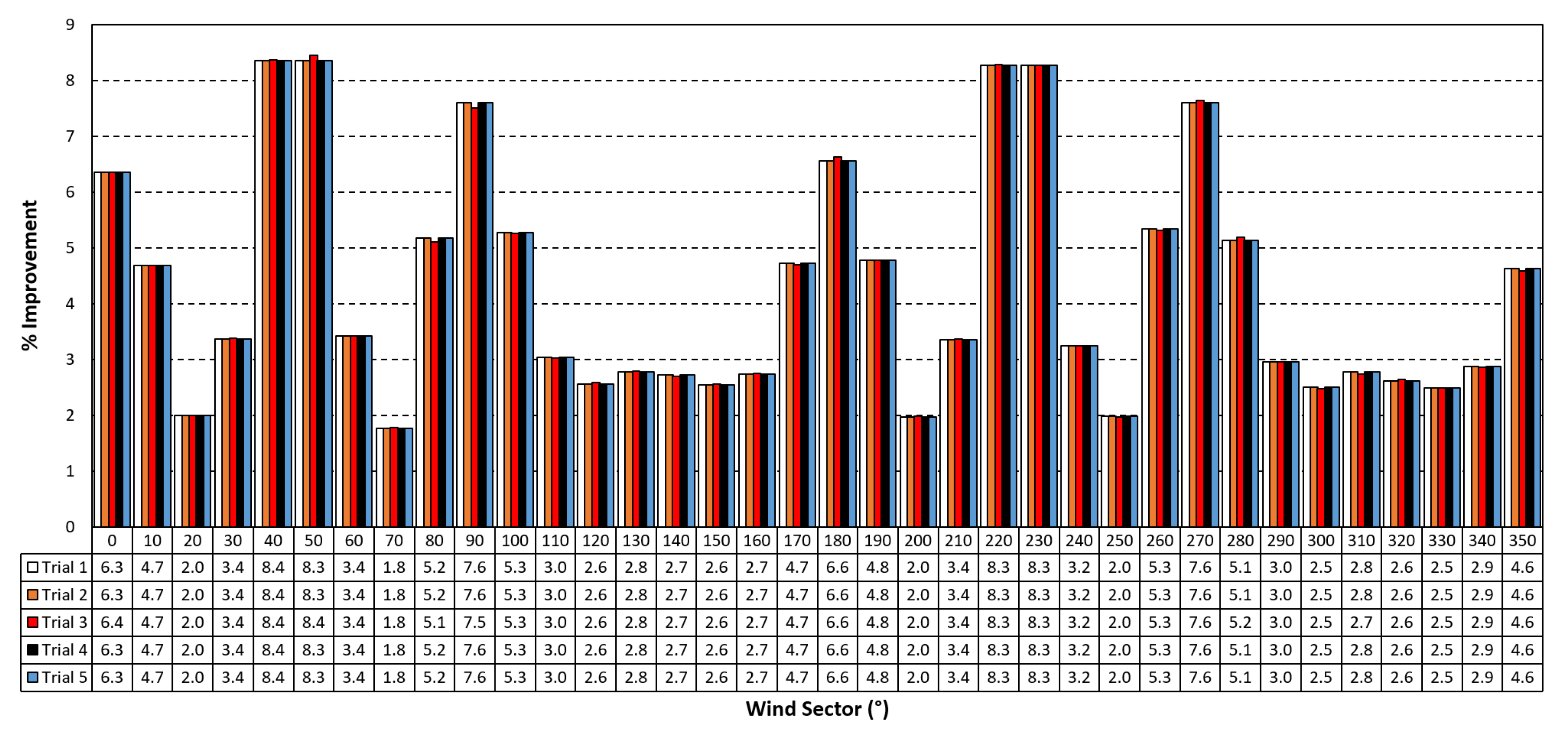
4.3. Solution Reproducibility
Randomness is an inherent part of the proposed RS algorithm. To test the RS algorithm’s sensitivity to initial seeds, five trials were performed to demonstrate that the algorithm is able to explore the solution space and that the solution quality is insensitive of initial guesses. The results are shown in Figure 5, and two observations can be made. First, potential improvement is strongly dependent on wind direction. In particular, it is clear that production improvements are greatest when winds are blowing from cardinal and intercardinal directions, when turbines are aligned due to the structured-grid nature of the layout. Second, in each of the five trials, the improvements are nearly identical for all wind direction sectors. At first glance, this was very surprising as this implied that the RS algorithm is able to converge to similar objective values with different initial guesses. Upon closer inspection of the five solutions, it is likely that this type of problem has multiple local optima with similar solution quality and that the RS algorithm is able to adequately explore the solution space.
4.4. Solution Quality
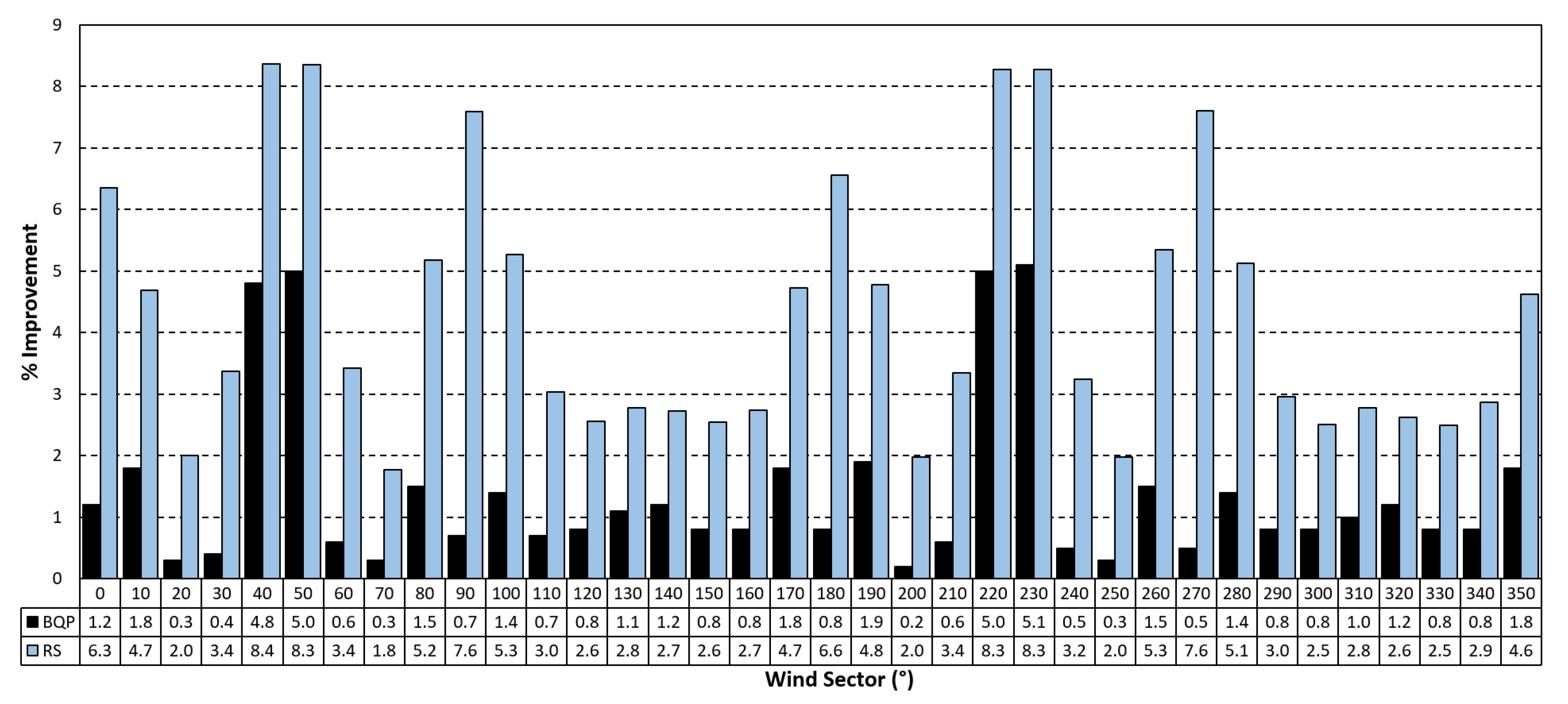
To the best of the authors’ knowledge, the only existing parametric studies on wake steering is the work by Kuo et al. [59], which illustrated that the potential of wake steering is a function of wind farm density. That work employed a binary quadratic programming (BQP) formulation. The formulation only allows turbines to yaw a discrete number of angles. Although this discrete formulation limited the quality of solutions, the formulation allowed well-developed mathematical programming methods to be applied, as the BQP solution is known to be optimal. This work can be compared to the BQP formulation in terms of solution quality. Table 4 shows the power density and the average percent improvement of the proposed work and the BQP model, and Figure 6 shows the comparison for different wind direction sectors at m. Two observations can be drawn from Table 4. First, as power density increases with turbine diameter, production improvement also increased, as previously observed in the work by Kuo et al. Second, the production improvement from RS algorithm significantly outperforms the BQP model. There are two reasons for this, (1) although the RS algorithm restricts yawing within a range of incremental angle for each iteration, it does not restrict turbines from yawing beyond that range. For example, even if is restricted to for each iteration, it is possible for a turbine to have a final yaw angle of after a number of iterations. However, this is not the case for the BQP formulation, where the range of angle is a global constraint. (2) The RS algorithm permits a more dynamic range of angles (e.g. varying values), while the BQP formulation only allows a predefined set of angles throughout the optimization process.
4.5. Sensitivity to Wind Direction
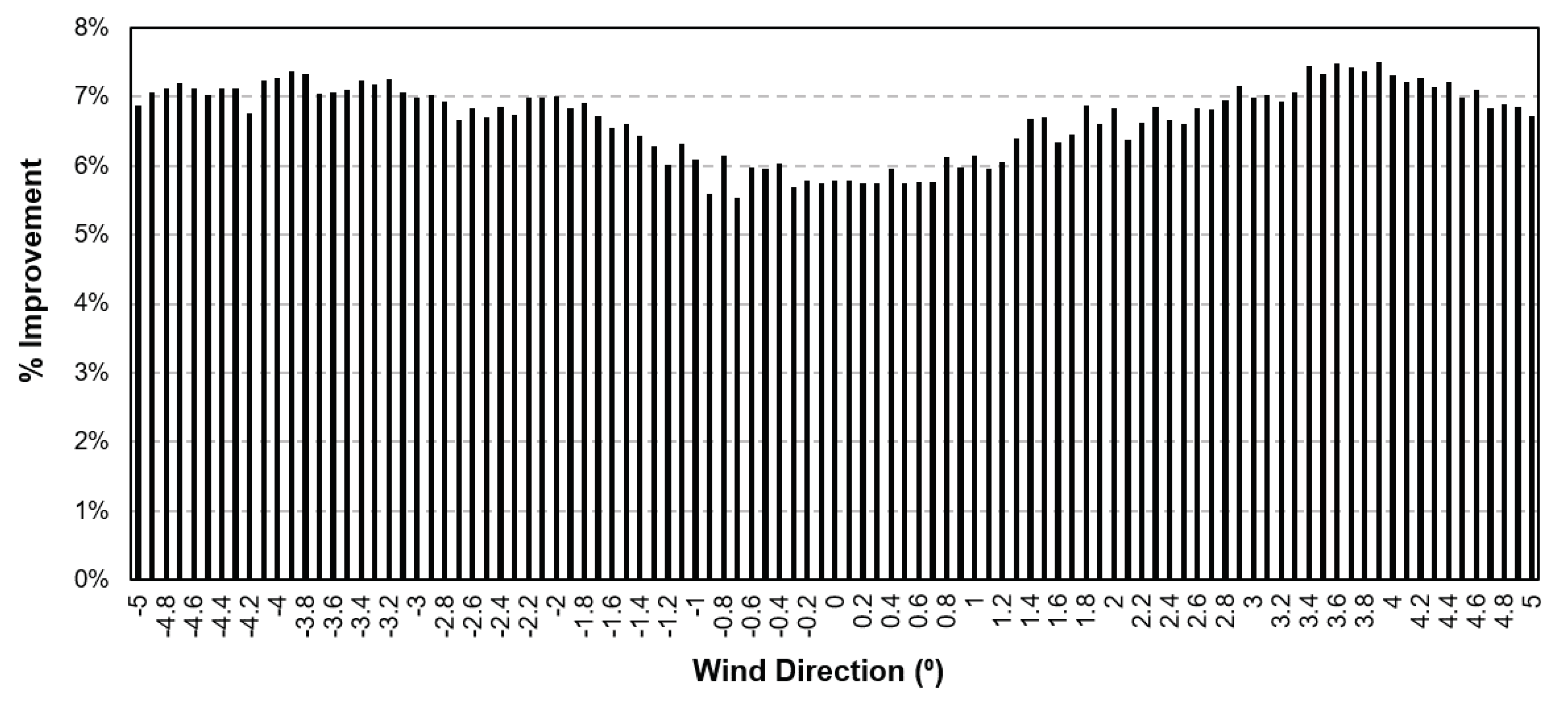
It is known that wake effects are very sensitive to changing wind directions, thus in this work, we perform simulations at resolution, then the results are averaged over 10 degree wind sectors. This approach is important as this particular wind farm layout is very structured such that turbines are mostly aligned in certain angles. This means that if wakes from upstream turbines are directly aligned with downstream turbines due to perfect alignment with wind direction, then upstream turbines would need to yaw significantly to reduce wake interactions downstream. This would also reduce overall gains as upstream turbines would produce less power as a result of larger yaw angles. If the wind is slightly misaligned with turbine positions, then improvements from yaw optimization should be larger. We illustrate this sensitivity by presenting the percentage improvement at wind sector, or wind directions from to at increment, shown in Figure 7. As discussed, it is clear that when wind direction moves away from (perfect alignment due to structured layout), the percent improvement from yaw optimization increases as turbines move out of perfect alignment from incoming wind. Although in this work, the approach of averaging the solutions at increment is performed, it is not possible in practice to change the yaw angles for every change in wind direction. Furthermore, there is no guarantee that a near-optimal solution for one particular wind direction will be a near-optimal solution within the wind sector. Thus, the future research direction is to develop a robust yaw optimization model, similar to that of the robust wind farm layout optimization model developed [17] for varying wind directions, and that the proposed RS algorithm can be used to solve the robust model.
5. Conclusions
This paper describes a random search algorithm capable of optimizing yaw angles of wind turbines. A series of tests have been conducted to understand the algorithm’s performance in terms of computational cost and solution quality. The proposed RS algorithm has been shown to significantly outperform previous work of a BQP formulation solved using a state-of-the-art mathematical programming solver, and the production improvement is tripled compared with BQP algorithm. Through the empirical study, the following observations have been made, (a) The quality of solutions is consistent and is reproducible over multiple runs with minor variations; (b) The solution quality is dependent on the range of yaw angles and the percentage of turbines yawed in each iteration; (c) During optimization process, it is more preferable to have larger range of yaw angle at the beginning and gradually tighten the range as the process continues to renew the results; (d) The optimal range of the percentage of turbines yawed in each iteration is between 5% and 50%; and (e) Near-optimal solutions (<1% of best known solutions) can be found within 500 iterations, and that excellent (<2% of best known solutions) solutions can be found under 300 iterations. While testing the capabilities of the proposed algorithm, four observations related to wind farm yaw optimization were made. First, as power density increases, the potential to improve production through yaw optimization increases. Second, good solutions are likely to be plentiful and are not unique. Third, yaw optimization can further improve power production in an optimized layout. Finally, yaw optimization is sensitive to changes in wind direction, so robust yaw optimization considering varying wind direction should be considered in future work.
Author Contributions
Conceptualization, N.L., H.S. and J.K.; methodology, N.L., H.S. and J.K.; software, J.K. and K.P.; validation, J.K. and K.P.; formal analysis, J.K., K.P. and H.S.; investigation, J.K., K.P., H.S. and N.L.; resources, J.K. and N.L.; data curation, K.P. and J.K.; writing–original draft preparation, J.K., K.P. and N.L.; writing–review and editing, J.K., H.S. and N.L.; visualization, K.P. and J.K.; supervision, J.K., H.S. and N.L.; project administration, J.K. and N.L.; funding acquisition, J.K. and N.L. All authors have read and agreed to the published version of the manuscript.
Funding
This research was funded by the Center of Energy and Sustainability at California State University, Los Angeles, and the National Science Foundation under Award No. HRD-1547723.
Acknowledgments
The authors would like to thank Y. Curtis Wang at the California State University, Los Angeles for his computing support.
Conflicts of Interest
The authors declare no conflict of interest.
References
- Barthelmie, R.J.; Hansen, K.; Frandsen, S.T.; Rathmann, O.; Schepers, J.G.; Schlez, W.; Phillips, J.; Rados, K.; Zervos, A.; Politis, E.S.; et al. Modelling and measuring flow and wind turbine wakes in large wind farms offshore. Wind Energy 2009, 12, 431–444. [Google Scholar] [CrossRef]
- Kusiak, A.; Song, Z. Design of wind farm layout for maximum wind energy capture. Renew. Energy 2010, 35, 685–694. [Google Scholar] [CrossRef]
- Du Pont, B.L.; Cagan, J. An extended pattern search approach to wind farm layout optimization. J. Mech. Des. 2012, 134, 081002. [Google Scholar] [CrossRef]
- Chowdhury, S.; Zhang, J.; Messac, A.; Castillo, L. Unrestricted wind farm layout optimization (UWFLO): Investigating key factors influencing the maximum power generation. Renew. Energy 2012, 38, 16–30. [Google Scholar] [CrossRef]
- Serrano Gonzalez, J.; Burgos Payan, M.; Riquelme Santos, J. Wind farm optimal design including risk. In Proceedings of the International Symposium on Modern Electric Power Systems (MEPS), Wroclaw, Poland, 20–22 September 2010; pp. 1–6. [Google Scholar]
- Kwong, W.; Zhang, P.; Romero, D.; Moran, J.; Morgenroth, M.; Amon, C. Wind farm layout optimization considering energy generation and noise propagation. In Proceedings of the ASME 2012 International Design Engineering Technical Conferences & Computers and Information in Engineering Conference, Chicago, IL, USA, 12–15 August 2012; pp. 1–10. [Google Scholar]
- Chen, L.; MacDonald, E. Considering Landowner Participation in Wind Farm Layout Optimization. J. Mech. Des. 2012, 134, 084506. [Google Scholar] [CrossRef]
- Chen, L.; MacDonald, E. A system-level cost-of-energy wind farm layout optimization with landowner modeling. Energy Convers. Manag. 2014, 77, 484–494. [Google Scholar] [CrossRef]
- Zhang, P.Y.; Romero, D.A.; Beck, J.C.; Amon, C.H. Solving Wind Farm Layout Optimization with Mixed Integer Programming and Constraint Programming. In International Conference on AI and OR Techniques in Constriant Programming for Combinatorial Optimization Problems; Springer: Berlin, Germany, 2013; pp. 284–299. [Google Scholar]
- Turner, S.; Romero, D.; Zhang, P.; Amon, C.; Chan, T. A new mathematical programming approach to optimize wind farm layouts. Renew. Energy 2014, 63, 674–680. [Google Scholar] [CrossRef]
- Fagerfjäll, P. Optimizing wind farm layout: more bang for the buck using mixed integer linear programming. Master’s Thesis, Chalmers University of Technology and Gothenburg University, Gothenburg, Sweden, 2010. [Google Scholar]
- Donovan, S. An improved mixed integer programming model for wind farm layout optimisation. In Proceedings of the 41th Annual Conference of the Operations Research Society, Wellington, New Zealand, 30 November 2006. [Google Scholar]
- Chowdhury, S.; Zhang, J.; Messac, A.; Castillo, L. Characterizing the influence of land configuration on the optimal wind farm performance. In Proceedings of the ASME 2011 International Design Engineering Technical Conferences & Computers and Information in Engineering Conference (IDETC/CIE 2011), No. DETC2011-48731, ASME, Washington, DC, USA, 28–31 August 2011. [Google Scholar]
- Pérez, B.; Mínguez, R.; Guanche, R. Offshore wind farm layout optimization using mathematical programming techniques. Renew. Energy 2013, 53, 389–399. [Google Scholar] [CrossRef]
- Wagner, M.; Day, J.; Neumann, F. A fast and effective local search algorithm for optimizing the placement of wind turbines. Renew. Energy 2013, 51, 64–70. [Google Scholar] [CrossRef] [Green Version]
- Kuo, J.Y.; Romero, D.A.; Beck, J.C.; Amon, C.H. Wind farm layout optimization on complex terrains–Integrating a CFD wake model with mixed-integer programming. Appl. Energy 2016, 178, 404–414. [Google Scholar] [CrossRef]
- Zhang, P.Y.; Kuo, J.Y.; Romero, D.A.; Chan, T.C.; Amon, C.H. Chapter 28: Robust Wind Farm Layout Optimization. In Advances and Trends in Optimization with Engineering Applications; SIAM: Philadelphia, PA, USA, 2017; pp. 367–375. [Google Scholar]
- Kuo, J.Y.; Romero, D.A.; Amon, C.H. A mechanistic semi-empirical wake interaction model for wind farm layout optimization. Energy 2015, 93, 2157–2165. [Google Scholar] [CrossRef]
- Antonini, E.G.; Romero, D.A.; Amon, C.H. Continuous adjoint formulation for wind farm layout optimization: A 2D implementation. Appl. Energy 2018, 228, 2333–2345. [Google Scholar] [CrossRef]
- Guirguis, D.; Romero, D.A.; Amon, C.H. Gradient-based multidisciplinary design of wind farms with continuous-variable formulations. Appl. Energy 2017, 197, 279–291. [Google Scholar] [CrossRef]
- Feng, J.; Shen, W. Modelling wind for wind farm layout optimization using joint distribution of wind speed and wind direction. Energies 2015, 8, 3075–3092. [Google Scholar] [CrossRef] [Green Version]
- Adaramola, M.; Krogstad, P.Å. Experimental investigation of wake effects on wind turbine performance. Renew. Energy 2011, 36, 2078–2086. [Google Scholar] [CrossRef]
- Jiménez, Á.; Crespo, A.; Migoya, E. Application of a LES technique to characterize the wake deflection of a wind turbine in yaw. Wind Energy 2010, 13, 559–572. [Google Scholar] [CrossRef]
- Fleming, P.; Gebraad, P.M.; Lee, S.; van Wingerden, J.W.; Johnson, K.; Churchfield, M.; Michalakes, J.; Spalart, P.; Moriarty, P. Simulation comparison of wake mitigation control strategies for a two-turbine case. Wind Energy 2015, 18, 2135–2143. [Google Scholar] [CrossRef]
- Boorsma, K. Power and Loads for Wind Turbines in Yawed Conditions: Analysis of Field Measurements and Aerodynamic Predictions; ECN: Schagen, The Netherlands, 2012. [Google Scholar]
- Bastankhah, M.; Porté-Agel, F. Experimental and theoretical study of wind turbine wakes in yawed conditions. J. Fluid Mech. 2016, 806, 506–541. [Google Scholar] [CrossRef]
- Vollmer, L.; Steinfeld, G.; Heinemann, D.; Kühn, M. Estimating the wake deflection downstream of a wind turbine in different atmospheric stabilities: An LES study. Wind Energy Sci. 2016, 1, 129–141. [Google Scholar] [CrossRef] [Green Version]
- Gebraad, P.; Thomas, J.J.; Ning, A.; Fleming, P.; Dykes, K. Maximization of the annual energy production of wind power plants by optimization of layout and yaw-based wake control. Wind Energy 2017, 20, 97–107. [Google Scholar] [CrossRef] [Green Version]
- Annoni, J.; Bay, C.; Taylor, T.; Pao, L.; Fleming, P.; Johnson, K. Efficient optimization of large wind farms for real-time control. In Proceedings of the 2018 Annual American Control Conference (ACC), Milwaukee, WI, USA, 27–29 June 2018; pp. 6200–6205. [Google Scholar]
- Munters, W.; Meyers, J. Dynamic strategies for yaw and induction control of wind farms based on large-eddy simulation and optimization. Energies 2018, 11, 177. [Google Scholar] [CrossRef] [Green Version]
- Archer, C.L.; Vasel-Be-Hagh, A. Wake steering via yaw control in multi-turbine wind farms: Recommendations based on large-eddy simulation. Sustain. Energy Technol. Assess. 2019, 33, 34–43. [Google Scholar] [CrossRef]
- Fleming, P.; Ning, A.; Gebraad, P.M.; Dykes, K. Wind plant system engineering through optimization of layout and yaw control. Wind Energy 2016, 19, 329–344. [Google Scholar] [CrossRef] [Green Version]
- Wu, Y.T.; Porté-Agel, F. Atmospheric Turbulence Effects on Wind-Turbine Wakes: An LES Study. Energies 2012, 5, 5340–5362. [Google Scholar] [CrossRef]
- Boersma, S.; Doekemeijer, B.; Gebraad, P.M.; Fleming, P.A.; Annoni, J.; Scholbrock, A.K.; Frederik, J.; van Wingerden, J.W. A tutorial on control-oriented modeling and control of wind farms. In Proceedings of the 2017 American Control Conference (ACC), Seattle, WA, USA, 24–26 May 2017; pp. 1–18. [Google Scholar]
- Qian, G.W.; Ishihara, T. A New Analytical Wake Model for Yawed Wind Turbines. Energies 2018, 11, 665. [Google Scholar] [CrossRef] [Green Version]
- Gebraad, P.M.; Teeuwisse, F.; Van Wingerden, J.; Fleming, P.A.; Ruben, S.; Marden, J.; Pao, L. Wind plant power optimization through yaw control using a parametric model for wake effects - a CFD simulation study. Wind Energy 2016, 19, 95–114. [Google Scholar] [CrossRef]
- Howland, M.F.; Bossuyt, J.; Martínez-Tossas, L.A.; Meyers, J.; Meneveau, C. Wake structure in actuator disk models of wind turbines in yaw under uniform inflow conditions. J. Renew. Sustain. Energy 2016, 8, 043301. [Google Scholar] [CrossRef] [Green Version]
- Lopez, D.; Kuo, J.; Li, N. A novel wake model for yawed wind turbines. Energy 2019, 178, 158–167. [Google Scholar] [CrossRef]
- Kuo, J.; Rehman, D.; Romero, D.A.; Amon, C.H. A novel wake model for wind farm design on complex terrains. J. Wind Eng. Ind. Aerodyn. 2018, 174, 94–102. [Google Scholar] [CrossRef]
- Shapiro, C.R.; Gayme, D.F.; Meneveau, C. Modelling yawed wind turbine wakes: A lifting line approach. J. Fluid Mech. 2018, 841. [Google Scholar] [CrossRef] [Green Version]
- Park, J.; Law, K. A bayesian optimization approach for wind farm monitoring and power maximization. In Proceedings of the 6th International Conference on Structural Health Monitoring of Intelligent Infrastructure, Hong Kong, China, 9–11 December 2013. [Google Scholar]
- González, J.S.; Payán, M.B.; Santos, J.R.; Rodríguez, Á.G.G. Maximizing the overall production of wind farms by setting the individual operating point of wind turbines. Renew. Energy 2015, 80, 219–229. [Google Scholar] [CrossRef]
- Gebraad, P.M.; van Wingerden, J.W. Maximum power-point tracking control for wind farms. Wind Energy 2015, 18, 429–447. [Google Scholar] [CrossRef]
- Gebraad, P.M.; Teeuwisse, F.; van Wingerden, J.W.; Fleming, P.A.; Ruben, S.D.; Marden, J.R.; Pao, L.Y. A data-driven model for wind plant power optimization by yaw control. In Proceedings of the 2014 American Control Conference, Portland, OR, USA, 4–6 June 2014; pp. 3128–3134. [Google Scholar]
- Ahmad, M.A.; Hao, M.R.; Ismail, R.M.T.R.; Nasir, A.N.K. Model-free wind farm control based on random search. In Proceedings of the 2016 IEEE International Conference on Automatic Control and Intelligent Systems (I2CACIS), Selangor, Malaysia, 22–22 October 2016; pp. 131–134. [Google Scholar]
- Howland, M.F.; Lele, S.K.; Dabiri, J.O. Wind farm power optimization through wake steering. Proc. Natl. Acad. Sci. USA 2019, 116, 14495–14500. [Google Scholar] [CrossRef] [PubMed] [Green Version]
- Ahmad, T.; Basit, A.; Ahsan, M.; Coupiac, O.; Girard, N.; Kazemtabrizi, B.; Matthews, P.C. Implementation and Analyses of Yaw Based Coordinated Control of Wind Farms. Energies 2019, 12, 1266. [Google Scholar] [CrossRef] [Green Version]
- Ahmad, T.; Basit, A.; Anwar, J.; Coupiac, O.; Kazemtabrizi, B.; Matthews, P.C. Fast Processing Intelligent Wind Farm Controller for Production Maximisation. Energies 2019, 12, 544. [Google Scholar] [CrossRef] [Green Version]
- Rotea, M.A. Dynamic programming framework for wind power maximization. IFAC Proc. Vol. 2014, 47, 3639–3644. [Google Scholar] [CrossRef] [Green Version]
- Dar, Z.; Kar, K.; Sahni, O.; Chow, J.H. Windfarm power optimization using yaw angle control. IEEE Trans. Sustain. Energy 2016, 8, 104–116. [Google Scholar] [CrossRef]
- Kingma, D.P.; Ba, J. Adam: A method for stochastic optimization. arXiv 2014, arXiv:1412.6980. [Google Scholar]
- Mittal, A. Optimization of the Layout of Large Wind Farms using a Genetic Algorithm. Ph.D. Thesis, Case Western Reserve University, Cleveland, OH, USA, 2010. [Google Scholar]
- Herbert-Acero, J.F.; Franco-Acevedo, J.R.; Valenzuela-Rendón, M.; Probst-Oleszewski, O. Linear wind farm layout optimization through computational intelligence. In MICAI 2009: Advances in Artificial Intelligence; Springer: Berlin, Germany, 2009; pp. 692–703. [Google Scholar]
- Bilbao, M.; Alba, E. GA and PSO Applied to Wind Energy Optimization. In Proceedings of the CACIC Conference Proceedings, Jujuy, Argentina, 5–9 October 2009. [Google Scholar]
- Chen, L.; MacDonald, E. A new model for wind farm layout optimization with landowner decisions. In Proceedings of the ASME 2011 International Design Engineering Technical Conferences & Computers and Information in Engineering Conference, Washington, DC, USA, 28–31 August 2011. [Google Scholar]
- González, J.S.; Gonzalez Rodriguez, A.G.; Mora, J.C.; Santos, J.R.; Payan, M.B. Optimization of wind farm turbines layout using an evolutive algorithm. Renew. Energy 2010, 35, 1671–1681. [Google Scholar] [CrossRef]
- Dahlberg, J.; Montgomerie, B. Research program of the Utgrunden demonstration offshore wind farm. In Final Report Part 2, Wake Effects and Other Loads; Swedish Defense Research Agency: Kista, Sweden, 2005; pp. 2–17. [Google Scholar]
- Schreck, S.; Schepers, J. Unconventional Rotor Power Response to Yaw Error Variations; Journal of Physics: Conference Series; IOP Publishing: Bristol, UK, 2014; Volume 555, pp. 1–12. [Google Scholar] [CrossRef]
- Kuo, J.; Li, N.; Shen, H. A Feasibility Study of Wind Farm Yaw Angle Optimization. In Proceedings of the ASME 2019 International Mechanical Engineering Congress & Exposition, Salt Lake City, UT, USA, 11–14 November 2019; pp. 1–10. [Google Scholar]
- Grady, S.; Hussaini, M.; Abdullah, M. Placement of wind turbines using genetic algorithms. Renew. Energy 2005, 30, 259–270. [Google Scholar] [CrossRef]
- Van Laarhoven, P.J.; Aarts, E.H. Simulated Annealing. In Simulated Annealing: Theory and Applications; Springer: Berlin, Germany, 1987; pp. 7–15. [Google Scholar]
Figure 1.
plane of Gaussian wake as described by Qian and Ishihara [35].
Figure 1.
plane of Gaussian wake as described by Qian and Ishihara [35].

Figure 2.
plane of Gaussian wake as described by Qian and Ishihara [35].
Figure 2.
plane of Gaussian wake as described by Qian and Ishihara [35].

Figure 3.
Proposed random search algorithm. Note that power output is abbreviated as PO.

Figure 4.
Optimal layout from Grady et al. [60].
Figure 4.
Optimal layout from Grady et al. [60].

Figure 5.
Percent improvement in power production by wind direction sector at with five different initial random seeds.
Figure 5.
Percent improvement in power production by wind direction sector at with five different initial random seeds.

Figure 6.
Percent improvement in power production by wind direction sector, comparing proposed random search (RS) algorithm and binary quadratic programming (BQP) model [59] for m.
Figure 6.
Percent improvement in power production by wind direction sector, comparing proposed random search (RS) algorithm and binary quadratic programming (BQP) model [59] for m.

Figure 7.
Percent improvement in power production between wind directions to at increment for m.


Table 1.
Wind farm parameters.
| Parameters | Values |
|---|---|
| Domain Size (km × km) | 2 × 2 |
| Hub Height (m) | 60 |
| Rotor Diameter (m) | 60 |
| Number of Turbines | 39 |
| Rated Turbine Power (kW) | 518 |
| Wind Speed (m/s) | 12 |
| Thrust Coefficient | 0.88 |
| Power coefficient | 0.5 |
| Power Curve | Theoretical |
| Turbulence Intensity | 0.035 |
| Wind Direction Sector | 36, every |
Table 2.
Percent improvement in power with differing values at m with northerly wind ( direction sector, 10 degree sector, averaged over increment) after 1000 iterations and five trials. Best five objective values are underlined and the best average is boldfaced.
Table 2.
Percent improvement in power with differing values at m with northerly wind ( direction sector, 10 degree sector, averaged over increment) after 1000 iterations and five trials. Best five objective values are underlined and the best average is boldfaced.
| Value of | Trial 1 | Trial 2 | Trial 3 | Trial 4 | Trial 5 | Average |
|---|---|---|---|---|---|---|
| () | (%) | (%) | (%) | (%) | (%) | (%) |
| 2 | ||||||
| 5 | ||||||
| 10 | ||||||
| 20 | ||||||
Table 3.
Percent improvement in objective value (from unyawed solution) as function of number of iterations with varying F values at m with northerly wind ( direction sector, 10 degree sector, averaged over increment), averaged over 5 trials, with and . Best objective value at each iteration is underlined.
| Value of | Number of | Iteration | |||||
|---|---|---|---|---|---|---|---|
| Turbines | 50 | 100 | 200 | 300 | 500 | 1000 | |
| 100 | 39 | 1.61% | 2.71% | 3.92% | 4.65% | 5.31% | 5.90% |
| 51.3 | 20 | 2.14% | 3.38% | 4.52% | 5.22% | 5.78% | 6.12% |
| 35.9 | 14 | 2.00% | 3.64% | 4.80% | 5.34% | 5.93% | 6.22% |
| 30.8 | 12 | 1.88% | 3.31% | 4.81% | 5.49% | 5.93% | 6.26% |
| 25.6 | 10 | 1.94% | 3.15% | 4.79% | 5.52% | 6.09% | 6.39% |
| 20.5 | 8 | 1.76% | 3.33% | 4.85% | 5.55% | 6.09% | 6.38% |
| 17.9 | 7 | 1.91% | 3.28% | 4.83% | 5.56% | 6.14% | 6.39% |
| 15.4 | 6 | 1.62% | 3.01% | 4.72% | 5.49% | 6.11% | 6.34% |
| 12.8 | 5 | 1.51% | 2.84% | 4.47% | 5.35% | 6.12% | 6.36% |
| 10.3 | 4 | 1.53% | 2.66% | 4.50% | 5.41% | 6.09% | 6.39% |
| 7.7 | 3 | 1.31% | 2.53% | 4.19% | 5.11% | 6.07% | 6.45% |
| 5.1 | 2 | 1.11% | 2.10% | 3.57% | 4.65% | 5.74% | 6.48% |
| 2.5 | 1 | 0.72% | 1.37% | 2.43% | 3.16% | 4.21% | 5.79% |
Table 4.
Power density and percent production improvement of layout from Grady et al. [60] using binary quadratic programming (BQP) model [59] compared with proposed random search (RS) algorithm.
| Turbine | Power Density | BQP Production | RS Production |
|---|---|---|---|
| Diameter (m) | (MW/km) | Improvement (%) [59] | Improvement(%) |
| 40 | 0.39 | 0.98 | |
| 60 | 1.45 | 4.25 | |
| 80 | 3.22 | 10.72 |
© 2020 by the authors. Licensee MDPI, Basel, Switzerland. This article is an open access article distributed under the terms and conditions of the Creative Commons Attribution (CC BY) license (http://creativecommons.org/licenses/by/4.0/).
Share and Cite
MDPI and ACS Style
Kuo, J.; Pan, K.; Li, N.; Shen, H. Wind Farm Yaw Optimization via Random Search Algorithm. Energies 2020, 13, 865. https://doi.org/10.3390/en13040865
AMA Style
Kuo J, Pan K, Li N, Shen H. Wind Farm Yaw Optimization via Random Search Algorithm. Energies. 2020; 13(4):865. https://doi.org/10.3390/en13040865
Chicago/Turabian StyleKuo, Jim, Kevin Pan, Ni Li, and He Shen. 2020. "Wind Farm Yaw Optimization via Random Search Algorithm" Energies 13, no. 4: 865. https://doi.org/10.3390/en13040865
Note that from the first issue of 2016, this journal uses article numbers instead of page numbers. See further details here.