 Miral S. Tawfik1*
 Amogh Subbakrishna Adishesha2Yuhan Hsi2
 Prakash Purswani3Russell T. Johns3,4Parisa Shokouhi5Xiaolei Huang2Zuleima T. Karpyn3,4
- 1Reservoir Engineering and Simulation, Chevron Technical Center, Houston, TX, United States
- 2Information Science and Technology, The Pennsylvania State University, University Park, PA, United States
- 3The Energy Institute, The Pennsylvania State University, University Park, PA, United States
- 4John and Willie Leone Family Department of Energy and Mineral Engineering, The Pennsylvania State University, University Park, PA, United States
- 5Department of Engineering Science and Mechanics, The Pennsylvania State University, University Park, PA, United States
Digital rock physics has seen significant advances owing to improvements in micro-computed tomography (MCT) imaging techniques and computing power. These advances allow for the visualization and accurate characterization of multiphase transport in porous media. Despite such advancements, image processing and particularly the task of denoising MCT images remains less explored. As such, selection of proper denoising method is a challenging optimization exercise of balancing the tradeoffs between minimizing noise and preserving original features. Despite its importance, there are no comparative studies in the geoscience domain that assess the performance of different denoising approaches, and their effect on image-based rock and fluid property estimates. Further, the application of machine learning and deep learning-based (DL) denoising models remains under-explored. In this research, we evaluate the performance of six commonly used denoising filters and compare them to five DL-based denoising protocols, namely, noise-to-clean (N2C), residual dense network (RDN), and cycle consistent generative adversarial network (CCGAN)—which require a clean reference (ground truth), as well as noise-to-noise (N2N) and noise-to-void (N2V)—which do not require a clean reference. We also propose hybrid or semi-supervised DL denoising models which only require a fraction of clean reference images. Using these models, we investigate the optimal number of high-exposure reference images that balances data acquisition cost and accurate petrophysical characterization. The performance of each denoising approach is evaluated using two sets of metrics: (1) standard denoising evaluation metrics, including peak signal-to-noise ratio (PSNR) and contrast-to-noise ratio (CNR), and (2) the resulting image-based petrophysical properties such as porosity, saturation, pore size distribution, phase connectivity, and specific surface area (SSA). Petrophysical estimates show that most traditional filters perform well when estimating bulk properties but show large errors for pore-scale properties like phase connectivity. Meanwhile, DL-based models give mixed outcomes, where supervised methods like N2C show the best performance, and an unsupervised model like N2V shows the worst performance. N2N75, which is a newly proposed semi-supervised variation of the N2N model, where 75% of the clean reference data is used for training, shows very promising outcomes for both traditional denoising performance metrics and petrophysical properties including both bulk and pore-scale measures. Lastly, N2C is found to be the most computationally efficient, while CCGAN is found to be the least, among the DL-based models considered in this study. Overall, this investigation shows that application of sophisticated supervised and semi-supervised DL-based denoising models can significantly reduce petrophysical characterization errors introduced during the denoising step. Furthermore, with the advancement of semi-supervised DL-based models, requirement of clean reference or ground truth images for training can be reduced and deployment of fast X-ray scanning can be made possible.
Background and Introduction
Micro-computed tomography (MCT) is a non-destructive technique used to visualize the internal structure of objects in a variety of disciplines including medicine, dentistry, tissue engineering, aerospace engineering, geology, and material and civil engineering (Orhan, 2020). The physical principle behind this technique is that X-rays attenuate differently as they penetrate through different materials depending on their density and atomic mass (Knoll, 2000; Attix, 2004; Ritman, 2004; Hsieh, 2015). This makes MCT an ideal tool for characterizing multiphase materials such as rocks with fluid phases of different densities.
The use of MCT imaging is becoming increasingly indispensable in several disciplines, including geotechnical and petrophysical characterization and understanding multiphase flow in porous media. Wang et al. (1984) first adopted medical CT imaging to monitor the injectant front to understand the effect of pore structure heterogeneity on oil recovery and interactions between oil and injected fluid in a Berea sandstone. However, medical CT imaging soon proved inadequate in describing the underlying pore-scale phenomena responsible for multiphase flow behavior in porous media (Cromwell et al., 1984). Therefore, high-resolution MCT imaging was used to obtain quantitative pore-scale information about structure–function relationships (Jasti et al., 1993). They characterized the 3D pore structure in a glass bead pack and three Berea sandstone samples to determine whether topological properties such as pore connectivity and phase features of individual fluid phases such as saturation can be resolved. Micro-computed tomography has since been successfully used for quantifying a wide range of petrophysical properties such as volume fraction for porosity and saturation quantification, specific surface area (SSA), pore- and blob-size distributions, in-situ contact angles, interface curvatures for local capillary pressures, grain sphericity, angularity, roughness as well as phase connectivity (Sharma and Yortsos, 1987; Prodanović and Bryant, 2006; Karpyn et al., 2010; Herring et al., 2013; Landry et al., 2014; Larpudomlert et al., 2014; Berg et al., 2016; Klise et al., 2016; Scanziani et al., 2017; Chen et al., 2018; Tawfik et al., 2019; McClure et al., 2020). The accuracy with which we can estimate these pore-scale properties affect our ability to explain and predict multiphase fluid flow in porous media. For example, pore-network modeling, which is used in a variety of digital rock studies to explain and predict macroscopic transport properties such as absolute permeability, relative permeability, and capillary pressure, uses simplified pore structures composed of a network of pores and throats, which can be directly extracted from the MCT images (Valvatne and Blunt, 2004; Jia et al., 2007; Dong et al., 2009; Mostaghimi et al., 2013; Berg et al., 2016; Zahaf et al., 2017; Raeini et al., 2019). Similarly, Lattice Boltzmann simulation of multiphase flow is used to estimate the same transport properties but on real pore structures by directly using the binarized MCT images as input (Grader et al., 2010; Andrä et al., 2013; Landry et al., 2014; Liu et al., 2014; Armstrong et al., 2016; Kakouei et al., 2017; Li et al., 2018). The accuracy of the model predictions thus depends on the accuracy of processing the images that feed into these models.
Despite the fast-paced advances in MCT imaging, there are several factors that introduce noise to MCT images limiting the image quality and feature detectability. Those limitations can hinder our ability to accurately identify structure-function relationships and predict fluid flow behavior, which is essential in several applications including CO2 storage, aquifer remediation, and hydrocarbon recovery. Some of the inherent limitations of MCT imaging include photon statistics, balance between representative elementary volume and resolution or feature detection, and partial volume consideration (Van Stappen, 2018). Apart from image resolution, there are numerous artifacts that arise during image acquisition. The prominent ones include photon starvation, detector saturation also known as ghosting, central rotation artifact, cone-beam effect, metal artifact, cupping artifact, streaks and dark bands, under-sampling, poor contrast, beam hardening, scatter, and ring artifacts (Boas and Fleischmann, 2012). These imaging artifacts result in different forms of noise in a CT image. Though noise in MCT has not been fully profiled, many studies including Diwakar and Kumar (2018) and Lee et al. (2018) have attempted to profile the noise distributions through known statistical distributions. The most prevalent noise forms follow Poisson and Gaussian distributions. There are several other forms of noise including fractal noises like Perlin noise, periodic noise from helical sampling and finally random noise that may occur due to the change in X-ray quanta for multiple subject densities. Gaussian and Poisson noise are the most common types of noise observed in MCT images. Gaussian noise is additive and signal independent. Poisson noise is a consequence of low photon count, and results in random thin bright and dark streaks that appear preferentially along the direction of greatest attenuation (Boas and Fleischmann, 2012). The low photon count coupled with the error in quantization of the received photons leads to a mixture noise-model, which is a combination of Poisson and Gaussian distributions. Perlin noise is a pseudo-random texture gradient noise which is generated using octaves of noise flow vectors along with frequency and amplitude parameters to simulate spatially interpolated textures (Perlin, 1985). The granularity and texture of the noise profile in low quality (LQ) CT images can be captured by Perlin noise. Bae et al. (2018) showed that using Perlin noise profile to augment a lung CT dataset resulted in higher classification accuracy indicating that the features extracted from Perlin noise augmented images matched those of certain low-dose CT scans with lung conditions.
Mathematically, denoising is an inverse ill-posed problem where noisy data is a sparse representation of the real data and a unique solution for its restoration does not necessarily exist (Fan et al., 2019). For an exact solution to the problem, a priori knowledge of the types of noise, variance of noise within an image and along the image stack would be required. This information is usually not readily available. The basic principle behind most of the traditional spatial domain denoising filters is noise removal based on spatial correlation between an input pixel gray value and its neighboring pixels. Those filters can be classified into linear and non-linear filters. Linear filters are spatially invariant filters that output pixel values as a linear combination of the input pixel value and its neighborhood. Examples of linear filters include Gaussian and mean filters, which are optimal for Gaussian noise. However, linear filters tend to blur edges and blur small features. Conversely, non-linear filters can be spatially invariant like the median filter, or spatially variant like the anisotropic diffusion (AD) filter (Huang et al., 1979; Perona and Malik, 1990). Another approach to denoise MCT images involves machine-learning-based models. As such, the objective is to find the parameters that act on the sparse noisy data to obtain the closest representation of the clean signal. Several works in literature have approached this parameter estimation through the use of classic machine learning and modern neural network-based models (Tian et al., 2020). Improvements in the DL denoising field result from a clearer understanding of the specific noise forms and improvements in the architecture of neural networks. The literature points to three specific architectures, namely U-Nets, Residual Networks, and Generative Adversarial Networks (GANs), that have been established for addressing common noise forms including Poisson, Gaussian, and their mixtures which are predominant in CT images (Kulathilake et al., 2021).
Deep learning (DL) powered computer vision has seen phenomenal improvement since the introduction of AlexNet in 2012 (Krizhevsky et al., 2017). However, adaptation of imaging techniques for porous media is still work in progress. Kamrava et al. (2019) trained a 20-layer feedforward neural network using synthetic data generated by the stochastic cross-correlation-based simulation (CCSIM) algorithm and found that neural networks perform better compared to bi-cubic interpolation for image super-resolution while the synthetic data further improved the model's generalizability. Sidorenko et al. (2021) implemented an encoder-decoder network for denoising MCT images obtained from tight sandstone samples. The authors compared the effect of different loss functions and found that the least absolute deviation (L1) loss gave a better result in terms of peak signal to noise ratio (PSNR) and structural similarity index measure (SSIM) when compared to the least square errors (L2) loss, SSIM loss, and Visual Geometry Group (VGG) perceptual loss. Recently, Alsamadony et al. (2021) acquired low-exposure and high-exposure CT scans on the same carbonate sample and compared denoising performance using a pre-trained very deep super resolution (VDSR) network against a shallow U-Net. They demonstrated that DL-based image processing can improve image quality; and that pre-trained VDSR network with fine-tuning tends to out-perform VDSR trained from scratch. Wang et al. (2021) reviewed various DL applications in pore-scale imaging and modeling, including image segmentation, image super-resolution, petrophysical property prediction, flow simulation, as well as common convolutional neural network (CNN) architectures and various types of GANs for image generation. However, the discussion on image denoising was brief. A summary of findings from select literature on image denoising with applications in digital rock physics is provided in Table 1.

Table 1. A summary of selected publications that report on MCT imaging in the digital rock physics domain, highlighting the commonly used denoising methods.
The literature survey reveals a need for a comprehensive comparison of denoising approaches for petrophysical applications. Existing studies mostly utilize non-learnable filters and rely on visual inspection to evaluate the effect of image denoising. The lack of quantitative metrics, both standard and physics-based, cause errors during this critical image processing step to remain largely unquantified. Finally, none of the reported studies consider the impact of denoising techniques on downstream tasks such as image segmentation and petrophysical property estimation, which is often the ultimate goal of quantitative imaging.
In this paper, we address these research gaps and compare the performance of traditional (user-based) denoising methods against more sophisticated DL-based denoising methods. Four types of models are considered in this study: (a) commonly used filters such as the Gaussian, non-local means (NLM), Median etc., (b) fully supervised models including the noise-to-clean (N2C), residual dense network (RDN), and cycle consistent generative adversarial network (CCGAN), (c) semi-supervised models that use a portion of clean reference images for learning, and (d) completely unsupervised techniques like the noise-to-noise (N2N) and noise-to-void (N2V). We evaluate the performance of the different denoising models using both qualitative and quantitative analyses against an independent ground truth. We also compare computational resource requirements and ease of implementation of the different methods and provide recommendations. From quantitative comparison, we show the utility of physics-informed evaluation based on petrophysical property estimation. From this exercise, we address the following research questions: can sophisticated denoising protocols yield a reasonable characterization of a saturated porous medium using fast X-ray scanning with low-exposure time? Can we use a reduced number of, or no clean reference images and still yield accurate petrophysical characterization estimates using low-exposure MCT images?
Methodology
Image Acquisition
In this section, we briefly describe the experiment conducted by Niu (2021) to generate the datasets used in this study. The MCT images used in this study are of a fritted Robu-type glass (borosilicate) filter procured from Adam & Chittenden Scientific Glass Cooperation. This porous medium was selected as a proxy for real rocks to minimize changes that typically take place in real rock samples when fluids are injected, such as dissolution, which can alter the results of the study. The core sample properties are given in Table 2.
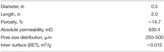
Table 2. Properties of the porous core sample (Niu, 2021).
The experimental procedure consisted of wrapping the core sample in a heat shrink jacket and placing it in an X-ray transparent Core Lab biaxial FCH series core holder (CoreLab, 2021; https://www.corelab.com/cli/core-holders/x-ray-core-holder-fch-series). This core holder is made of an aluminum body wrapped in carbon fiber composite, which reduces the holder's X-ray absorption capacity during scanning. The porous medium is saturated with high salinity brine that has a composition representative of a saline aquifer (Tawfik et al., 2019). Brine was pre-equilibrated with CO2 at 1,500 psi and 45°C before being used to saturate the core. The core sample was then flooded with supercritical CO2 (scCO2) at a pore pressure of 1,180 psi and temperature of 41.7 ± 0.2°C (107.06 ± 0.36°F), as well as confining pressure of 1,430 ± 50 psi. The confining pressure was applied by injecting deionized water into the annular space of the core holder. The high pore pressure and temperature enabled the maintenance of scCO2 conditions.
The MCT images were acquired using a GE v|tome|x L300 multi-scale nano/microCT system, using the 300 kV X-ray tube. Two datasets were acquired at the same voxel resolution of 15 μm: a high-quality (HQ) scan, where more exposure time was allowed to reduce noise. The second dataset was a low-quality (LQ) scan which was under the same experimental conditions, using the same scanning parameters except for exposure time, where less scanning time (~7.5 times less) was needed to produce a noisier version of the HQ dataset. The HQ dataset is used in this study as a ground truth to evaluate the different denoising methods and compare the petrophysical properties computed using the different denoised datasets. The HQ dataset is also used as a clean reference dataset to train the model for some of the DL denoising algorithms, which are discussed later in this section. The scanning details for both datasets are presented in Table 3. The sinograms generated during image acquisition were reconstructed using GE's proprietary GPU-based reconstruction software datos|x 2 reconstruction.

Table 3. MCT scanning parameters.
Selection and Implementation of Denoising Methods
The datasets obtained from the scans contain 2,024 32-bit images. Pre-processing of the datasets involved extracting a cylindrical sub-volume to eliminate the core holder and heat shrink jacket. Additionally, the top 103 and bottom 490 slices were removed to eliminate the cone-beam effect, which is typically observed at the top and bottom of the scan volume.
Non-learnable, Traditional Denoising Filters
Numerous filtering algorithms have been developed for reducing image noise to make the gray-scale CT images ready for the image segmentation step, after which feature extraction and quantitative analysis is carried out. In this study, we focus on the errors incurred particularly during the denoising step. Denoising may take place before image reconstruction by taking advantage of existing statistical models of noise, derived from an understanding of its physical origin. However, due to missing visual perception, operations performed on a sinogram might have unpredictable effects on real features post reconstruction (Matrecano et al., 2010). On the other hand, post-reconstruction filters are pixel-to-pixel transformations of an image. This transformation is based on the gray-scale intensity of each pixel and its neighboring pixels (Machado et al., 2013). They can be classified as low-pass or high-pass filters; a low-pass filter is used for image smoothing, whereas a high-pass filter is typically used for image sharpening. Some of the most commonly used filters include Gaussian filter, median filter, NLM, and AD filter.
The Gaussian filter is a low-pass filter that uses a Gaussian function. Applying this filter involves convolving an image with a Gaussian function, which may result in a blurrier image. A median filter is also a low-pass smoothening filter. It replaces the gray-scale value of each pixel with the median of its neighborhood. The neighborhood is pre-specified by the user as 6 faces, 18 edges, or 26 vertices. The process may be repeated to further smooth the image. The median Filter usually works well when images contain non-Gaussian noise and/or very small artifacts. The NLM filter first proposed by Buades et al. (2005) assumes the noise to be white noise. The value specified for the target voxel is a weighted-average of neighboring voxels within a user-specified search window. The weights are determined by applying a Gaussian kernel based on the similarity between the neighborhoods. The AD filter (Weickert, 1996) also known as the Perona-Malik diffusion, aims to reduce image noise within each phase while preserving edges and boundaries between phases. Typically, a diffusion stop criterion that exceeds the variation within a given phase is set to identify when diffusion should no longer take place to terminate diffusion and preserve edges. If this stop criterion is set to the maximum difference between voxel intensity values, diffusion never stops and the AD filter converges to a simple isotropic Gaussian filter. Some of the other used filters applied include Bilateral, SNN, Total variance, Nagao, Kuwahara, BM3D, Minimum, and Maximum filters.
The image processing software Avizo (v2020) was used to implement the simple filters, including the Gaussian, median, NLM, AD, bilateral, and SNN filters. For the Gaussian filter, the standard deviation was set to two voxels, and the kernel size was set to nine voxels in each direction. The median filter neighborhood was set to 26 (vertex neighborhood), and a total of three iterations are performed. The NLM filter was implemented using the adaptive-manifolds-based approach (Gastal and Oliveira, 2012). The search window was specified to be 500 voxels, and the local neighborhood was set to four. A large enough search window is selected to increase the chances of finding similar structures and phases. The local neighborhood value was determined such that it is similar in size to the fine structures that can be found in the image. Spatial standard deviation (which determines the relationship between how fast the similarity value decreases as distance between the target and neighboring voxel increases), was set to five. Similarly, the intensity standard deviation (which determines the relationship between how fast the similarity value decreases based on voxel intensities) was set to 0.2. For the AD filter, a total of five smoothing iterations per image is performed, with the diffusion stop threshold set to 0.048. That is, if the difference between the target voxel value and the value of its neighboring six voxels exceeds this stop threshold value, diffusion will not occur, hence preserving and enhancing phase interfaces. The bilateral filter parameters were kernel size = 3 and similarity = 20. Finally, for the SNN filter a kernel size of 3 was used. It is evident that these simple filters rely heavily on the user and their experience which lend themselves to likely bias. As such, there is a need for non-user-based denoising protocols.
Deep Learning Denoising Methods
A few notable DL-based denoising algorithms have been selected based on their architecture and input requirements. The most common architectures for encoder-decoder based denoising are U-Nets, GANs and RDNs. U-Nets are a sequence of contracting and expanding convolution blocks (forming a “U” shape) originally proposed by Ronneberger et al. (2015) for the purpose of biomedical image segmentation. U-Nets have the ability to accumulate hierarchical features at multiple resolutions and maintain sharpness throughout the decoding process (Diwakar and Kumar, 2018). Residual dense networks, on the other hand, are inspired by the neural connections present in a human brain. Here, output of a convolution block is combined with its input to help train deeper neural networks and maintain a version of the original input features. Residual dense networks have lately shown that accumulating features through local and global residual learning can significantly improve image restoration (Zhang et al., 2021). Finally, GANs, are a recent addition to the neural network family which are designed to generate data in a semi-supervised setting. The primary reason for the success of GANs, however, is its robust loss function which inherently accommodates several noise removal objectives like L1 distance, distribution matching etc. (Yang et al., 2018). This advantage proves essential in denoising tasks where noisy inputs have to be mapped to clean outputs.
In each of the above architectures, a state-of-the-art model has been identified and used for comparison against the traditional filter-based denoising techniques. Noise-to-clean is a U-Net proposed by Lehtinen et al. (2018) which learns to minimize a mean absolute error (MAE) distance between the denoised image and its corresponding clean reference. Similarly, residual dense network by Zhang et al. (2021) is a residual network aimed at improving fine-grained features in the restoration of noisy images. Cycle Consistent Generative Adversarial Denoising Network (CCGAN) by Kang et al. (2019) is multi-stage GAN network originally designed to denoise coronary CT images. The three models mentioned above use a supervised approach where they extract the 1:1 mapping between noisy and clean pixel intensities. However, in practice, clean reference MCT images are costly and hard to obtain, since this equates to higher X-ray exposure, longer scan durations and other noise prevention techniques which may not be cost- and/or time- efficient. For this reason, an evaluation involving unsupervised machine learning approaches is essential for practical purposes. In this direction, noise-to-noise by Lehtinen et al. (2018) is a reference-less approach based on a U-Net architecture and used for removing common noise forms present in images. Similarly, N2V is another unsupervised technique introduced by Krull et al. (2019), which uses pixel manipulations to infer the presence and removal of noise. Noise-to-noise ratio is a unique model which tries to estimate the unvarying signal behind varying noise realizations. This is intuitively similar to removing moving tourists in an unchanging scenic photo. The training for N2N requires the addition of a synthetic noise profile which matches low dose signal. For our purpose, we use a mixture of Poisson-Gaussian along with Perlin noise textures to simulate random noise. For the Poisson-Gaussian mixture, we first simulate the Poisson process using the pixel intensities as the mean (λ). We then scale this value with a Gaussian factor using mean (μ) of 0 and standard deviation (σ) that is randomly picked between 0 and 0.005. For the Perlin noise, we use a simplex model with scale set to 5, octaves to 6, persistence to 0.5, and lacunarity to 2.0 which showed the best match for the texture. Such profiles have been shown to emulate low-exposure noise in CT images (Lee et al., 2018). The model then learns to estimate the mean of the signal through several iterations. For test purposes, we do not add any noise and since the model is already accustomed to removing similar noise profiles, the denoising is successful.
Fully supervised and fully unsupervised DL models account for the best and worst-case scenarios of data availability, respectively. In this study, we propose new semi-supervised denoising models, where we use limited number of HQ high-exposure images to denoise a larger LQ low-exposure dataset. This can be applicable in several scenarios, including: (1) when the full length of a core sample needs to be scanned at a high resolution, yet resources in terms of time, availability, and money, are limited, and (2) when the processes or state of the core sample we are interested in visualizing changes quickly, and a fast, low exposure scan is deemed necessary (Gao et al., 2017), and (3) to avoid or minimize drift errors resulting from increased temperature of the experimental setup during longer scans, which leads to deviation of a feature from its original location due to mechanical and thermal stresses (Probst et al., 2016). Therefore, we extend the use of the N2N model to accommodate three HQ to LQ ratios where N2N25 is the scenario where 25% of the LQ data has a corresponding HQ reference image while 75% has no clean reference. Similarly, N2N50 and N2N75 indicate scenarios with a higher percentage of clean reference images. In the literature, fully supervised models use MAE between pixel intensities (L1 loss) to learn the mapping, whereas models like N2N and N2V, utilize a mean squared distance error (L2 loss). We propose a combination of the losses to reflect our semi-supervised task in training. For N2N25, we scale the L1 loss with a 0.25 weight and the L2 loss with a 0.75 weight. Similarly, for N2N50 and N2N75, we modify the weights to reflect the percentage of clean references. Using either L1 or L2 only yielded lower PSNR and SSIM values. Table 4 details the models and their specifications.
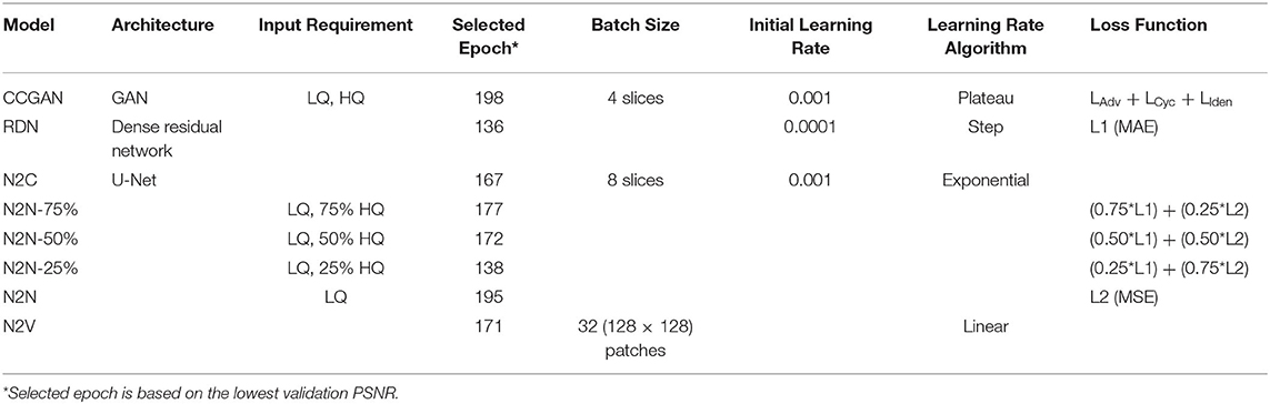
Table 4. Parameters selected for the DL-based denoising algorithms used in this study.
For the DL models, we split the training and testing data using a 80–20% non-overlapping split where 286 slices are randomly sampled from each of the LQ and HQ datasets and reserved for testing and validation, while the remaining 1,140 slices are used for training. The slices are reshaped to 512 × 512-pixel resolution using bicubic interpolation (Keys, 1981) in order to accommodate GPU memory limitations. After the model has been trained and evaluated, the original 800 × 800 resolution is obtained through similar bicubic interpolation. All the models are trained in accordance with their original implementation. Some hyperparameters are optimized to obtain the best possible performance from the model. Further details about the architecture, input requirements and choice of hyper-parameters like batch sizes, learning rate and number of epochs are provided in Table 4. We perform training over 200 epochs and use the ADAM optimization algorithm for all the models. We pick the epoch with the lowest validation PSNR in order to perform testing. Upon the completion of training, the evaluation is performed on the held out 286 slices from the test set. For all the models, ADAM optimization was used (Kingma and Ba, 2015).
Standard Quantitative Denoising Evaluation Metrics
Traditionally, image degradations that take place during acquisition, reconstruction, processing, and storage have been evaluated qualitatively by visual inspection and subjective assessment based on the assumption that human visual perception is highly adapted to extract structural information (Wang et al., 2004). However, as more data is being generated and more complex structures are being studied, it becomes increasingly difficult to rely on just human inspection. Thus, efforts to automate image quality assessment have been undertaken since 1972, when Budrikis developed one of the first quantitative measures to predict perceived image quality (Budrikis, 1972). These metrics have since evolved to match modern imaging and perceptual standards.
Peak Signal to Noise Ratio (PSNR)
Peak signal to noise ratio is a comparative metric widely used to determine noise degradation in an image with respect to a clean reference. Peak signal to noise ratio is an expression for the ratio between the maximum possible value (power) of a signal and the power of distorting noise that affects the quality of its representation. It is measured in decibels (dB) and the higher the PSNR, the better the image. Theoretically, PSNR for the HQ image is not defined and so it is manually set to 100 dB. In our setting, we calculate the PSNR on the test set which has not been used for training the models. The PSNR value reported for a model is averaged over the previously 286 held-out slices from the test set. The PSNR of the LQ slices act as a baseline for comparison.
Structural Similarity Index Measure (SSIM)
Unlike PSNR, SSIM is a perceptual metric which is not based on pixel intensities but rather on structural similarity between the denoised and the clean reference images (Wang et al., 2004). This is especially important when trying to evaluate fine-grained details and edges. It ranges from 0 to 1, where higher SSIM indicates a cleaner image. Similar to PSNR each of the SSIM values are calculated and averaged. The equation for the SSIM calculation is detailed in the Appendix in Supplementary Material.
Blurring Index
Many denoising algorithms focus on removing high-frequency components which correspond to noise. However, this leads to blurry images with fuzzy edges and high smoothness. Blurring index penalizes such images with a lower blurring index score. Occasionally, some DL models, smoothen regions based on expected intensity values leading to the removal of sharp high frequency noise elements. Though this is beneficial, the models obtain lower blurring index (BI) scores. The implementation of BI is detailed in the Appendix in Supplementary Material.
Contrast to Noise Ratio (CNR)
In grayscale images, a vital requirement of restoration models is the ability to separate foreground region intensities from the background noise. Contrast-to-noise ratio (CNR) is a reference-less metric which yields a higher value for higher contrasts and lower values for indistinguishable foreground and background regions. The higher the CNR, the cleaner the image, which makes it easier to segment the different phases. Our implementation follows Shahmoradi et al. (2016), where we identify six key regions of interest (ROI) including a background region from 10 random slices in the denoised test set. A detailed explanation of the CNR formula is provided in the Appendix in Supplementary Material.
Blind/Reference-Less Image Spatial Quality Evaluator (BRISQUE)
Blind/reference-less image spatial quality evaluator (BRISQUE) helps understand the presence of noise in an image without the use of a reference (Mittal et al., 2011). It relies on spatial statistics of the natural scene (NSS) model of locally normalized luminance coefficients in the spatial domain, as well as the model for pairwise products of these coefficients in order to extract spatially dense variances which occur in noisy images. We use the publicly available PyBRISQUE-1.0 software package (2020) for the implementation of this metric (https://pypi.org/project/pybrisque/).
Naturalness Image Quality Evaluator (NIQE)
Naturalness image quality evaluator (NIQE) unlike BRISQUE computes distortion specific features such as ringing, blur, and blocking to quantify possible losses of “naturalness” in the image due to the presence of distortions, thereby leading to a holistic measure of quality (Mittal et al., 2013). For this, we use the skvideo.measure.niqe package from the Scikit-Video library version 1.1.11 (Skvideo, 2013; http://www.scikit-video.org/stable/modules/generated /skvideo.measure.niqe.html). Each of the 286 slices are individually passed through the function and the scores are averaged for each model.
Physics-Informed Quantitative Denoising Evaluation Metrics: Petrophysical Characterization
Physics-informed denoising evaluation is performed through the estimation of petrophysical properties extracted from image data. To estimate these petrophysical properties, the denoised images need to be segmented to extract phase labels. In order to highlight the effect of different denoising approaches, and their effect on image-based rock and fluid property estimates, we used the same segmentation method on all denoised data. The segmentation method used was Ilastik1, a supervised machine-learning based segmentation tool that is built using a fast random forest algorithm (Sommer et al., 2011). The user manually provides a limited number of voxel labels for training. We maintain the same features among the different denoised datasets (Table 5). An almost equal number of marker voxels were selected for each of the three phases (solid/glass, brine, and scCO2). Also, the number of markers was kept to a minimum (~0.005% of sample voxels) to avoid overfitting. The same number of marker voxels per slice is maintained across all the datasets to minimize bias.
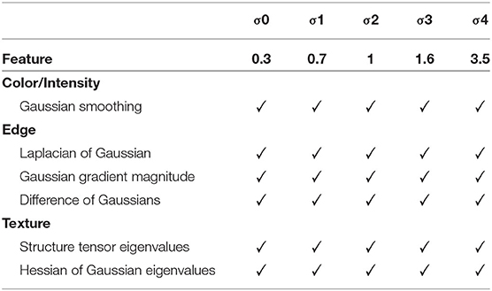
Table 5. Features selected for segmentation for the different datasets using ilastik.
The use of quantitative denoising evaluation metrics is a good practice over qualitative and subjective assessment of image quality. However, a HQ image as determined by standard denoising evaluation metrics may not necessarily render the most accurate estimate of petrophysical properties, either due to insufficient noise removal, or excessive filtering which results in information loss. Therefore, we evaluate the implemented denoising algorithms based on how various calculated petrophysical properties compare to those calculated using the HQ benchmark dataset. To achieve this, a toolbox was developed in Matlab R2019a to calculate different petrophysical properties, including (1) porosity, (2) saturation, (3) phase connectivity, which is represented by phase specific Euler number (phase Euler number divided by the phase volume), (4) phase SSA, which is calculated as the area of a given phase divided by its volume, (5) fluid-fluid interfacial area, (6) mean pore size, and (7) mean scCO2 blob volume. We also calculate phase fractions per slice along the length of the core.
Results and Discussion
In this section, we first describe the denoising results qualitatively by visual comparison of denoised datasets to the HQ ground truth images. Next, we present quantitative comparison results. The first set of quantitative comparison include standard metrics. Finally, we compare the quantitative petrophysical results of the denoised images post segmentation against the ground truth HQ segmented images.
Qualitative Evaluation of Denoising Methods
Figure 1 shows top view cross-sections from the HQ and the LQ data sets. The LQ image is evidently noisier than the HQ image. We have also marked regions to highlight spatial feature differences between the HQ and LQ images and associated implications for petrophysical property estimation. The red region shows that some small solid features can be inaccurately characterized as fluid, resulting in porosity estimation errors, while the green region demonstrates a blurry fluid-fluid interface in the LQ image, which can lead to errors in estimating fluid saturation and petrophysical properties pertaining to fluid–fluid interfaces. Similarly, the blue region shows an example where the solid phase can be falsely characterized as connected in the LQ image, while the HQ image shows some disconnection of the solid phase. This could result in errors in topological characterization, such as Euler number calculations for the solid phase.
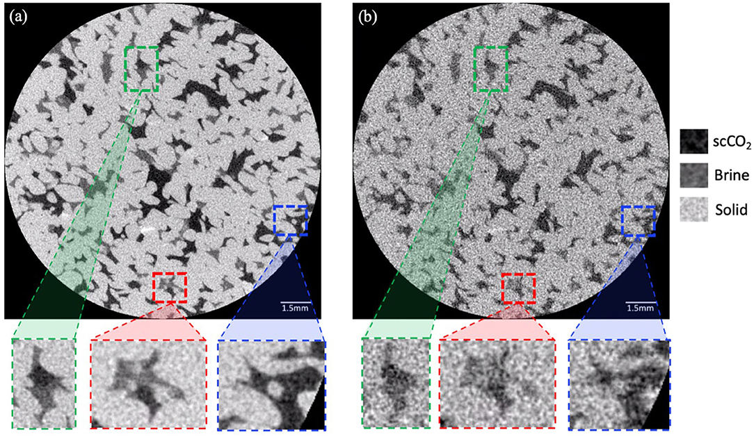
Figure 1. (a) Sample cross-sectional slice from the HQ dataset, (b) Sample cross-sectional slice from the LQ dataset. Dashed boxes represent spatial features that demonstrate differences between the two datasets. The red box represents an example region which can cause deviation in calculated porosity. The blue box represents an example region which can cause deviation in calculated connectivity. The green box represents an example region which can cause deviation in calculated saturation.
A cross-sectional image for each of the HQ dataset, LQ dataset and the denoised datasets are shown in Figure 2. Visually, the NLM filter results in an overall smoother image with significantly less variation within each phase (solid, brine, and scCO2), as it replaces the value of each voxel with the mean of similar voxels within the search window. The median and SNN filters also visually exhibit smoother phases, compared to the AD and bilateral filters. Conversely, the Gaussian filter expectedly results in image blurring, which can highly affect the accuracy of calculated interfacial petrophysical properties, such as interfacial area and mean interface curvature. The reference-based DL methods qualitatively show good performance compared to traditional filters. Noise-to-clean and CCGAN show a superior performance over RDN, with smoother phases and sharper edges. However, comparing the two models (N2C and CCGAN) with the HQ reference image, CCGAN resembles the reference image more closely in some features (highlighted in the blue circles), while N2C resembles the reference image more closely in other features (highlighted in the green circles). This exemplifies that qualitative or visual evaluation of denoising models is not a sufficient means of evaluation when deciding on the best denoising model to use. Reference-less DL methods (N2V and N2N) show little improvement compared to the LQ dataset. Finally, the semi-supervised DL methods show visually promising results, where the N2N-75% and N2N-50% show significant improvement compared to LQ.
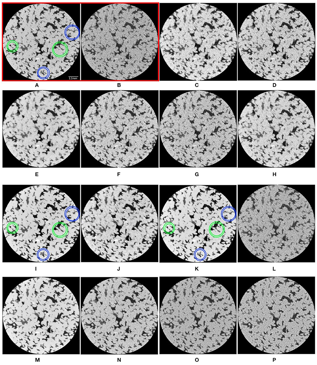
Figure 2. Qualitative comparison of the performance of the different denoising methods through example cross-sectional slices. (A), HQ reference; (B), LQ; (C),Gaussian; (D), Median; (E), Non-local means; (F), Anisotropic diffusion; (G), Bilateral; (H), Symmetric nearest neighbor; (I), Noise-to-clean; (J), Residual dense network; (K), Cycle consistent generative adversarial network; (L), Noise-to-void; (M), Noise-to-noise (75%); (N), Noise-to-noise (50%); (O), Noise-to-noise (25%); (P),Noise-to-noise.
The histogram representing the distribution of gray-scale intensities within a dataset can be used to qualitatively assess image quality. In our dataset, where we expect to see three phases—solid glass, brine, and scCO2, an ideal histogram would have three well-defined peaks with varying maximum voxel count, depending on the abundance of the phase represented by that peak in the imaged sample. The more distinguishable those peaks are, the sharper the phase boundaries and interfaces, and the easier the segmentation. Also, the smaller the spread of each peak, the smoother the bulk phase is (i.e., the phase is represented by less gray-scale values indicating a more homogeneous or smooth bulk phase). In Figure 3, we show the histograms of the HQ, LQ, and denoised datasets. The solid glass peak has the highest voxel count in all datasets, as expected, being the most abundant phase in our sample. We also observe a clear difference between the HQ and LQ datasets, where we can see three peaks in 3a, but only one visible peak in 3b, which makes the differentiation between scCO2 and brine more difficult. From the denoised dataset histograms, the supervised and semi-supervised DL denoising models perform better than traditional and un-supervised DL denoising methods. Also, we observe that the issue of fluid-fluid differentiation (where we can't see all three peaks) persists when using the bilateral, N2V, N2N25, and N2N denoising methods. We also observe that some denoising models possibly outperformed the HQ dataset where the three peaks are even more distinguishable, including N2C, RDN, CCGAN, and N2N75. Additionally, upon comparing 3i and 3k with 3j, we can see results consistent with our observations from Figure 2, where N2C and CCGAN have more well-defined and narrower peaks compared to RDN. Despite the additional insight obtained from inspecting the gray-scale intensity histograms, histograms alone cannot be used to infer image quality. The histogram indicates the distribution of pixel intensities but not their location. This calls for a more localized inspection of the images to assess how voxel spatial distribution impacts the accuracy of petrophysical property estimates.
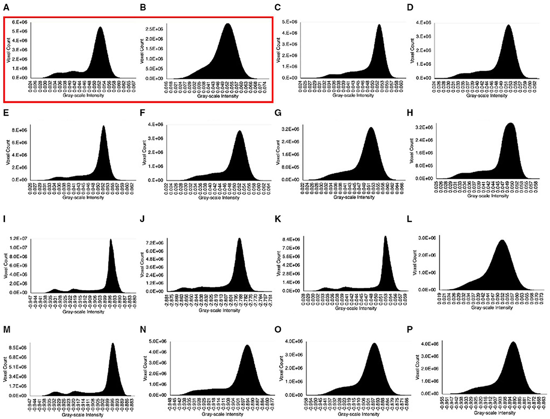
Figure 3. Qualitative comparison of the performance of the different denoising methods through gray-scale histograms.
Quantitative Evaluation of Denoising Methods
Figure 4 demonstrates a more quantitative method for evaluating the performance of the different denoising models using an intensity profile along a line A–A′. Here, we use N2C as an example. From this profile, we can obtain insights on the (1) smoothing effect within each phase by comparing the plateau of the noisy LQ dataset to that of the HQ and denoised dataset, and (2) contrast enhancement, which can be assessed by comparing the difference in intensities between the different phases. A larger difference implies an improvement in contrast, and finally (3) we can also assess phase boundary sharpness by calculating the steepness of the slope at each phase boundary. A steeper slope indicates a sharper boundary, which makes it more easily identifiable during image segmentation and petrophysical characterization. In Figure 4, we observe that the HQ profile exhibits oscillations within each phase, which shows that noise still exists in the HQ data, but the amplitude of those oscillations is smaller, which implies less noise and more homogeneous phases. We also observe slightly higher average intensity for the solid and brine phases in the HQ profile compared to the LQ profile. Additionally, we observe that N2C has improved the image quality on all three aspects: smoothing bulk phases, improving contrast between phases, and improving boundary sharpness. The scCO2-solid phase boundary has the most improvement in boundary sharpness with ~28% increase in slope.
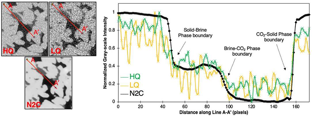
Figure 4. (Left) Example cross-sections through the high quality (HQ), low quality (LQ) and Noise-to-Clean (N2C) datasets. (Right) Normalized gray-scale values along a line (A-A′) passing through the solid, brine, and scCO2 phases in the example cross sections. Slopes at the phase boundaries are indicative of phase boundary sharpness for the HQ, LQ, and N2C profiles.
Example regions are highlighted in Figure 5a, following the workflow proposed by Shahmoradi et al. (2016) to assess local image quality using CNR. ROI-0 corresponds to the background which is used to calculate the CNR of other regions. ROI-1 corresponds to brine with no interfaces, while ROI-2 corresponds to the scCO2 phase, and ROI-3 corresponds to the solid phase. In addition, two interface regions, ROI-4, an interface between solid and brine and ROI-5, an interface between solid and scCO2 are also considered. We pick a random slice and indentify ROIs 1–5 in the next 22 consecutive slices. Figures 5b,c show localized average CNR values within bulk phases and at solid-fluid interfaces, respectively. We see that all denoising models, except for N2V, result in an improved CNR both in bulk phases and at interfaces. Supervised DL denoising models result in the largest CNR improvement, with N2C being a top performer. The N2N75 model also yields similar results as fully supervised denoising models, which is promising for cases where not all the HQ data is available. We also observe that the N2N25 model results in lower average CNR compared to N2N, which can be counter intuitive. However, this could be due to the inherent training objective of the model. The base N2N model estimates the mean of the signal and uses multiple noisy versions of the same signal to do so. However, when a small number of clean samples are provided, the network's estimate of the mean diverges from the expected value, which negatively affects learning. When provided with enough clean samples (50% or greater), the model converges to the mean more accurately compared to the base N2N or N2N25 versions. Comparing the improvement within bulk phases and at phase boundaries, we do not see a significant difference, indicating that all denoising methods improve contrast homogeneously throughout the image. Although quantitative, one limitation of the type of analysis performed in Figures 4, 5 is that they evaluate the performance of the denoising models locally, which requires manual selection of specific sites. A comprehensive denoising model performance evaluation is quantified using standard evaluation metrics detailed in Table 6.
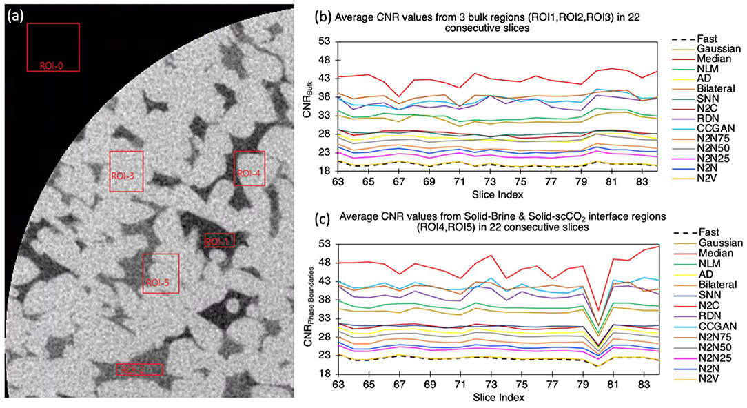
Figure 5. Comparison of contrast-to-noise (CNR) ratio for denoised datasets against noisy LQ dataset. (a) Example regions of interest (ROI 1–5) considered for bulk and edge CNR calculations are shown in red boxes. ROI 0 represents the background ROI against which contrast is calculated. (b) Average CNR of bulk phases (solid, brine, scCO2) in 22 slices, and (c) Average CNR of phase boundaries (solid-brine and solid-scCO2) in 22 slices.
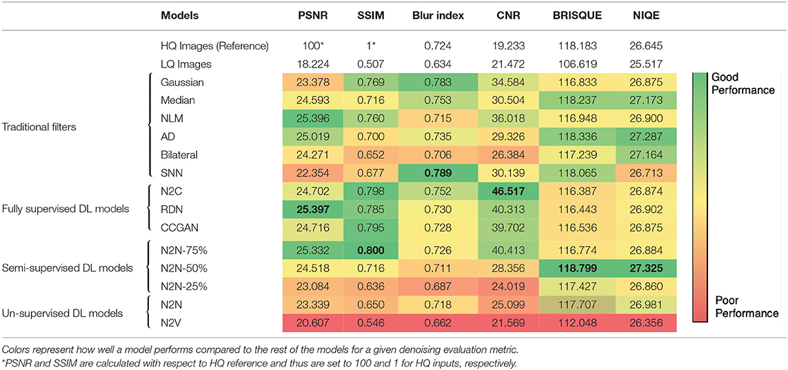
Table 6. Quantitative comparison of denoising algorithms using standard denoising evaluation metrics.
The CNR value reported here represents the average of the five individual CNR regions detailed earlier (Figure 5). Of the six metrics measured, the DL models performed the best in five of them. With Blur Index however, the metric measures the presence of sharpness which can be spiked by high frequency noise. The traditional filters failing to remove such noise achieve a misleading high blur-index score. Though the unsupervised models performed poorly, they were comparable to the traditional filter-based methods. Noise-to-noise ratio had the lowest values across all the metrics. It is also observed that PSNR values are generally low across all denoising methods. However, PSNR uses pixel distance and may incorrectly favor models that have higher resemblance to the HQ images rather than actual signal accuracy. The DL models tend to produce images that appear cleaner than the HQ image but score lower PSNR due to this reason. Residual dense network had the highest PSNR gain with an average increase of 7.173 dB. Though it might be possible for an image to obtain a high PSNR, SSIM penalizes structural anamolies like blurring, noise contamination, wavelet ringing, and blocking (caused by image compressions like JPEG) leading to lower SSIM scores.
Each evaluation metric points to unique capabilities of the models. For example, a high CNR obtained for N2C makes it ideal for segmentation tasks while a high SSIM obtained through N2N-75% model makes it favorable for CT image artifact removal task. The differences observed, however, between supervised DL-based models and N2N-75% in terms of SSIM are not statistically significant, meaning that they all perform equally well for this metric. N2N-50% produced the most natural looking images (NIQE) and can be used to generate additional synthetic clean samples when only 50% of clean data is available.
We also evaluated the denoising methods using physics-based metrics, or more specifically—petrophysical properties. To perform the petrophysical characterization, we first segmented the datasets. Figure 6 shows example segmented cross sections from the HQ and LQ datasets. It also shows a difference image, where the segmented LQ image was subtracted from the segmented HQ image. The percent mislabeling for each phase pair: brine-solid, scCO2-brine, and scCO2-solid is 2.46, 0.37, 1.57%, respectively. Based on the percent mislabeling of the denoised images, we see minor improvement compared to the LQ image. Similarly, image subtraction was performed between each of the denoised images and the HQ image. Noise-to-clean and N2N75 showed the most improvement especially in CO2-solid and brine-solid phase mislabeling. The differences are presumed to be mainly due to the difference in the amount of noise in each image since the user interference was kept to a minimum in the segmentation step. Further, the differences within this single image might seem subtle, but it has a significant effect on petrophysical characterization performed using the entire image stack. The full petrophysical characterization and error quantification against the ground truth is presented in Figure 7 and Table 7.
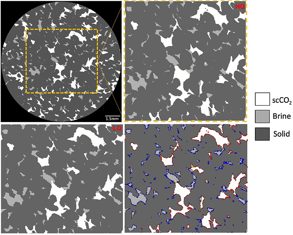
Figure 6. Example segmented HQ image using ilastik, and difference image |HQ–LQ| showing the mislabeling in LQ compared to the HQ image. Red, scCO2-solid mislabeling; Blue, brine-solid mislabeling; yellow, scCO2-brine mislabeling.
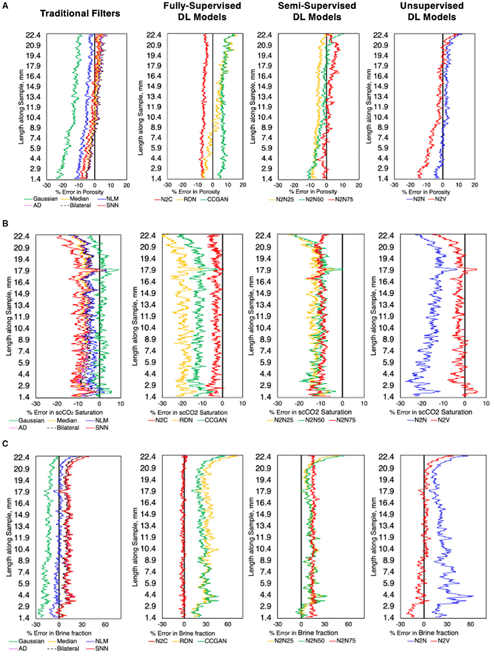
Figure 7. (A) Porosity, (B) scCO2 saturation, and (C) brine phase fraction percent error (relative to HQ) along the length of the core for the different denoising methods.
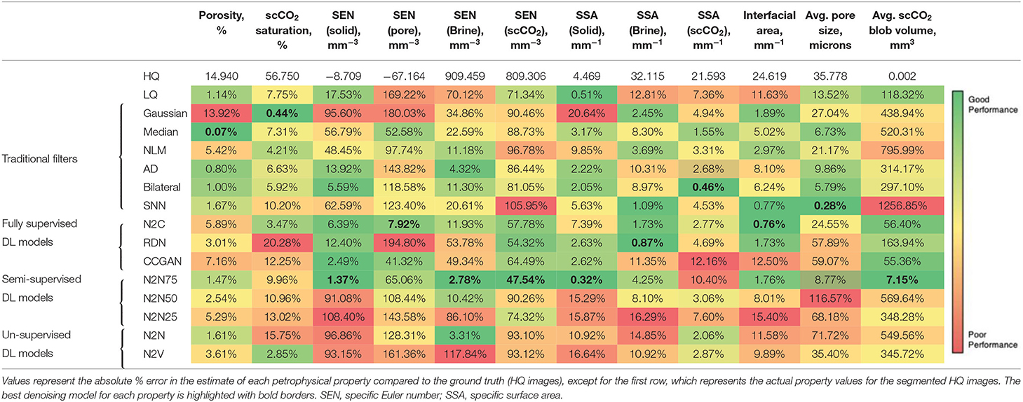
Table 7. Physics-based comparison of denoising algorithms using bulk and pore-scale petrophysical properties.
For petrophysical property estimations, we first consider bulk measures of phase fractions and saturations along the length of the core sample. Figure 7 shows the percent errors in porosity, scCO2 saturation, and brine fraction (measured as brine volume divided by the bulk volume for the sample space considered) profiles along the length of the sample for the different denoising methods post segmentation. The performance of denoising methods, namely, traditional methods, supervised, unsupervised, and semi-supervised DL-based methods are compared against the HQ dataset. Generally, most of the traditional and semi-supervised DL-based methods show closer results to the ground truth (Figure 7A). Out of the traditional filters, the median filter seems to have the closest porosity profile to the ground truth HQ dataset, followed by the AD and bilateral filters. Conversely, the Gaussian filter performed poorly, consistently underestimating porosity. Similarly, NLM, which is one of the most commonly used filters in the digital rock physics literature, underestimates porosity throughout the length of the core and has the second worst performance. Unlike their performance in terms of standard evaluation metrics (Table 6), supervised methods show poor performance, consistently underestimating porosity along the entire length of the sample. Additionally, the error is increasing toward the bottom of the sample in most denoising methods, especially Gaussian, RDN, and N2V methods. Upon inspecting the root cause of this, the original LQ dataset was noisier toward the bottom of the sample as evidenced by lower PSNR (Supplementary Figure 1A). This is mainly due to the aluminum container, covering the bottom half of the sample, used to fix the coreholder in place during the scan and avoid wobbling which can result in image blurring (Supplementary Figure 1B). The Gaussian filter, which is a linear spatially invariant filter, cannot resolve the noise variation along the sample. Residual dense network, a very deep network, could be overfitting the data and therefore less able to adjust to the varying noise along the sample, compared to other supervised models (N2C and CCGAN).
When comparing the CO2 saturation error profiles (Figure 7B), it is observed that traditional methods show close results, while most of the DL-based methods show poor performance when compared to the ground truth. Out of the traditional filters, SNN followed by median filters showed the most deviation from the ground truth. The Gaussian filter, on the other hand, had the closest results out of all the denoising models. Residual dense network and N2N significantly overestimate CO2 saturation. The supervised DL-based methods, except for N2C, show weak performance while the semi-supervised DL-based methods show slightly better performance. Noise-to-noise ratio, as an exception, shows the second-best performance of all methods, while RDN significantly underestimates scCO2 saturation. Larger error is seen at the top of the sample for all denoising methods except N2C and N2N75.
As the intermediate phase, brine fraction error profile is presented as opposed to brine saturation to account for errors that may result from misclassification of brine as solid or CO2 post-denoising (Figure 7C). Noise-to-clean, followed by NLM show the least deviation compared to the ground truth, whereas RDN, CCGAN, and N2N show a significant deviation. Noise-to-noise ratio also shows a surprisingly close match to the ground truth brine fraction profile. Overall, these results demonstrate that even within bulk property estimates, since differences occur at fluid-fluid and fluid-solid interfaces, consideration of both porosity and saturation errors is critical. Again, here we see that N2C and N2N75 are robust enough to maintain consistent performance throughout the sample even though the dataset has a spatially varying noise profile.
Table 7 summarizes the % errors associated with the estimates of bulk petrophysical properties, namely porosity and scCO2 saturation, as well as pore-scale properties including, specific Euler number, SSAs, interfacial area, average pore size and average scCO2 blob volume. These errors are quantified relative to the ground truth HQ images. The actual property estimates for the ground truth HQ images are presented in the first row of Table 7. Traditional filters like the median, AD and bilateral filters show an improved porosity estimate compared to the original LQ images, but the Gaussian filter results in the highest error for porosity (13.9%). This can be explained by the blurring caused by the Gaussian filter at phase interfaces, making it more difficult to locate boundaries, especially where the gray-scale intensities are less distinguishable like at the solid-brine interfaces. However, the Gaussian filter shows the best performance in terms of scCO2 saturation, which may be due to a larger surface area of the scCO2 phase being in contact with the solid phase rather than the brine phase, hence, enabling us to distinguish between the two phases more easily in terms of gray-scale intensity and labeling. The median filter on the other hand shows an opposite result where it exhibits better performance when estimating porosity and poorer performance in estimating scCO2 saturation. This can be explained by how a median filter works, where it involves replacing the gray-scale values of voxels within a user-specified window by their median value. This means that the small scCO2 blobs observed in the dataset in the bulk brine phase will be replaced with gray-scale values that resemble brine, leading to a lower scCO2 saturation (compared to HQ), but not affecting porosity as much. In general, most traditional filters perform better for bulk estimates of porosity and phase saturation, compared to DL-based methods.
For the pore-scale properties, we observe that supervised and semi-supervised methods show a better performance overall, except for scCO2 SSA and average pore size, where bilateral and SNN filters, respectively, show better performance. This can be attributed to the edge preserving nature of both the bilateral and SNN filters. For the scCO2 SSA, this allows fine-scale details like small scCO2 blobs observed in our dataset to be preserved, leading to a more accurate representation of phase boundaries and surfaces. Noise-to-clean and N2N75 perform well for most of the properties with ~10% error or less. Other methods like RDN and N2N25 perform poorly with errors as large as 348.28%. N2N75 also shows a more superior performance over N2C in terms of pore-scale estimates, which might not be expected due to the availability of more clean reference data to train the model for N2C, and the better overall standard metrics performance of N2C as shown in Table 6. However, it should be noted that the higher performance of N2N75 observed in Table 7 can be attributed to being a closer representation of the HQ data, which in our study is used as a ground truth. The HQ data is not an idealistic ground truth data, it has its own noise associated with it. Therefore, the comparison between N2C and N2N75 is limited by the amount of noise that is present in the HQ data which is the reference of comparison. We also observe one exception where RDN performs better than N2C and N2N75 in terms of brine SSA. This can be attributed to the ability of the RDN model to preserve high frequency details, which translates to a better ability to preserve high contrast phase boundaries and surfaces where SSA is calculated (Zhang et al., 2021).
Unsupervised DL-based methods (N2N and N2V) generally exhibit poor performance for most properties compared to other denoising methods including some of the traditional filters. This is in line with previous observations made during the analysis of the standard metrics in Table 6. Semi-supervised models, as expected, are performing better than unsupervised models. Counter-intuitively, adding additional information in low quantities (e.g., N2N25) can sometimes affect the model's capability to converge, leading to larger errors, as seen when we compare N2N and N2N25 errors for most properties. As we continue to add further information, the model manages to converge at the best possible parameters, which can also be seen for most properties when we compare N2N25, N2N50 and N2N75. We believe this is possible only after an optimum threshold percentage of clean reference images are provided.
To decide which denoising methods perform better in terms of bulk properties (porosity and scCO2 saturation) and pore-scale properties (SEN, SSA, interfacial area, average pore size and average blob volume), we sum up the absolute errors for each of the denoising methods for those two groups of properties. We also sum up all errors in Table 7 to identify the overall accuracy of each denoising method in terms of combined petrophysical characterization. Additionally, an aggregated standard evaluation metric is calculated by summing up the values in Table 6 for each method. The four aggregate metrics are presented in Supplementary Table 1. It is clear from Supplementary Table 1 that the denoising method selection should be highly dependent on the type of analysis of interest. For example, a denoising method that can offer accurate bulk properties might not be able to provide accurate pore-scale properties and vice versa. Aggregating the error percentages point out that N2N75 has the most consistent performance with the lowest overall error across both bulk and pore-scale properties while SNN has the highest error in estimating pore-scale properties and combined petrophysical properties. Noise-to-clean comes in a close second, however, it requires the complete HQ reference dataset. Among the traditional filters, the bilateral filter was the best performer across all aggregated metrics.
Computational Requirements of DL-Based Denoising Methods
Another important factor to consider when selecting a DL-based denoising model is computational requirements. Figure 8 shows the comparison of computational expenditure for the different DL-based models. Specifically, we compare the time required to process a single image slice of 800 × 800 pixels and the memory requirement which is computed from the parameters required for training. The system hardware available for implementing all models was the same (two Nvidia Quadro RTX 6000 GPU systems). Here, the comparison is presented against the traditional metric of PSNR to show how the models perform with the use of the required computational resources. We find that the supervised models, which show higher performance for PSNR, have substantially different computational needs, where RDN and CCGAN are approximately 5.6 and 8.6 times slower than N2C. Similarly, CCGAN is also found to be the most memory intensive primarily due to the training requirements of four individual networks while all other models share similar memory requirements (~1/6th that of CCGAN). When comparing the semi-supervised models, all three models (N2N25, N2N50, and N2N75) require the exact same computational resources both in terms of processing time and memory requirements. Finally, the unsupervised models (N2V and N2N) require similar memory requirements, but N2V is approximately four times slower than N2N. This could be attributed to the original PIP2 based implementation of the model. Overall, CCGAN is found to be the least computationally efficient, whereas N2C, N2N%, and N2N are the most efficient.
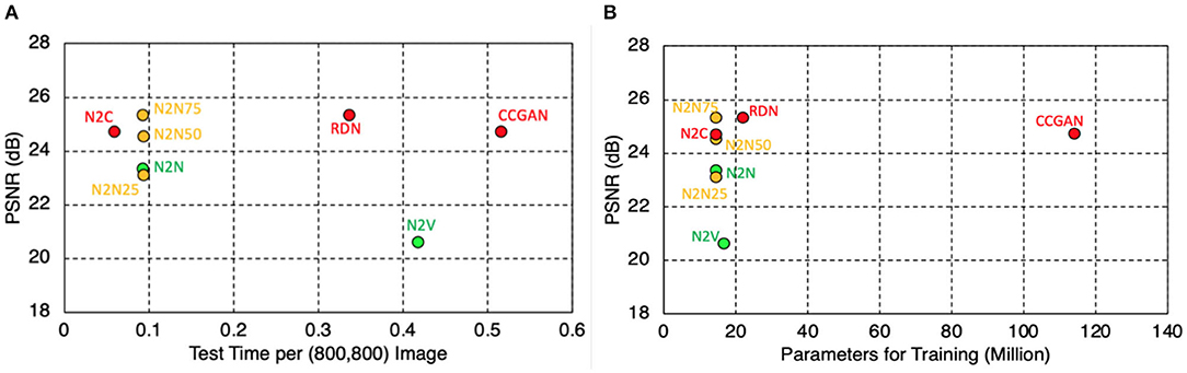
Figure 8. Comparison of computational requirement for the different DL-based denoising algorithms on 2 Nvidia Quadro RTX 6000 GPU systems, in terms of (A) computation time per (800,800) image, and (B) memory requirements as represented by parameters required for training. Red, fully supervised DL denoising models; yellow, semi-supervised DL denoising models; green, un-supervised DL denoising models.
Denoising Method Recommendation
Denoising is a mainstay pre-processing step performed to improve our ability to detect features and perform more accurate quantitative analyses using CT images. Comparing denoising methods through standard metrics and petrophysical property estimates helps us understand the use-cases in which certain models perform better. For example, despite performing well in terms of standard evaluation metrics, supervised DL models like N2C and RDN rely upon the availability of clean HQ data and such models cannot be used when such reference data is scarce or not available. Similarly, downstream tasks also determine the choice of denoising model. N2N50 can be recommended for generative tasks where additional synthetic data is required while N2C can be used if image segmentation is the proceeding step. Additionally, another important consideration is the availability of computational resources. Deep learning-based models require GPU-based systems to perform the training efficiently while traditional filters only require basic computational resources.
Based on the results we find that there is no one denoising method that ultimately performs better in all cases. Micro-computed tomography users are encouraged to adopt a similar evaluation workflow to derive an optimum denoising method that works best for their dataset(s) and use case. However, we present a high-level denoising model recommendation in Supplementary Table 2, based upon the different factors analyzed in this study. Though these factors influence the choice of a model individually, we list combinations of those factors to offer model recommendations for different scenarios. We derive the recommendations from Supplementary Table 1 and Figure 8 where we illustrate the superiority of some algorithms over others.
Conclusions and Future Work
Micro-computed tomography image artifacts and alterations resulting from using a non-tailored denoising protocol can result in inaccurate image-based characterization of porous media. In this paper, we present a comprehensive comparison of the performance of various image denoising methods which are broadly categorized as traditional (user-based) non-learnable denoising filters and DL-based methods. The DL-based methods are further sub-categorized depending on their reliance on reference data for the training process. Common architectures are used for supervised and unsupervised methods. We also proposed new semi-supervised denoising models (N2N75, N2N50, and N2N25) to assess the value of information and explore whether faster, lower exposure MCT images can partially substitute high-exposure datasets, which can be costly and can also hinder our ability to capture phenomena that occur at smaller time scales. The datasets used are those of a porous sintered glass core that has been saturated with brine and scCO2. We use both qualitative and quantitative evaluations to compare the performance of different denoising methods. For the latter, we consider standard denoising evaluation metrics, as well as physics-based petrophysical property estimates. The following conclusions are derived based on the analysis of our results
• Commonly used denoising filters in the digital rock physics literature, namely NLM and AD, show reasonable performance in terms of traditional denoising metrics like PSNR and SSIM. These methods also show reasonable estimates for the bulk petrophysical properties. However, when estimating pore-scale properties like phase connectivity, these methods could result in significant errors. NLM and SNN filters were found to perform least favorably in terms of pore-scale petrophysical estimates.
• Qualitative evaluation is usually used in the digital rock physics literature. However, we show that visual image quality is not sufficient to select an appropriate denoising algorithm.
• The selection of an optimum denoising model cannot solely depend on the visual quality of the denoised image, or even on the standard denoising evaluation metrics. Several factors need to be considered, including the availability of computational resources, and the post-processing analysis of interest. Physics-based petrophysical evaluation metrics are key in selecting a fit-for-purpose denoising method since a superior performance based on standard evaluation metrics may not necessarily indicate a superior performance in terms of petrophysical characterization accuracy. Additionally, there is no single best denoising algorithm across all petrophysical properties.
• The performance of the newly proposed semi-supervised methods, especially N2N75, is very promising considering that less high-exposure data can be used to achieve accurate petrophysical characterization, while significantly reducing scanning time and cost. This can also be useful in cases where the phenomenon being investigated has a short time-scale like chemical processes and pore-scale flow events. It can also help minimize rotational drift errors during scans.
• The unsupervised DL models, in general, showed the weakest performance both on standard and petrophysical evaluation metrics, with N2V giving the least favorable outcomes across most properties of interest.
• N2C (fully supervised) and N2N75 (semi-supervised with 75% HQ data) overall showed the most favorable outcomes. However, other supervised models like RDN and CCGAN and semi-supervised models like N2N50 and N2N25 showed weaknesses either on traditional metrics, petrophysical estimates, or computational requirements.
This study laid the groundwork for comparing and screening denoising methods for different use-cases within the digital rock physics domain. The following tasks are to be addressed in future work.
• Compare the performance of the different denoising methods using more complex petrophysical properties like surface roughness, tortuosity, interfacial curvature, in-situ contact angles, as well as fluid flow parameters such as absolute permeability, relative permeability, and capillary pressure. This comparison can enable optimum image processing workflow selection for creating accurate digital rocks that can be used for multiphase flow prediction and explanation.
• Optimize different denoising methods to accommodate different types of datasets. For that, we would need to first investigate the effect of porous medium structure complexity and image resolution on the performance of the different denoising methods.
• Use idealized simulated or synthetic ground truth reference images and test the effect of different types and levels of noise on the performance of each of the denoising methods, as well as combinations of the denoising methods.
• To identify the effect of noise in the HQ ground truth images on the conclusions drawn in this study, the same study can be conducted while using HQ datasets of varying exposure time.
• Optimize the newly proposed semi-supervised denoising models to determine the optimum threshold percentage of HQ high-exposure images that are needed while maintaining high accuracy of petrophysical analysis.
• Test the hypothesis of whether the sequential use of N2N25 can improve image quality to a point where accurate results are achievable.
• Explore the merits and drawbacks of sequential vs. co-learning in DL-based image processing, including reconstruction, denoising, and segmentation steps.
• Explore more novel unsupervised denoising methods to remove dependency upon HQ, high-exposure images and make use of less time and cost intensive scans for accurate petrophysical characterization.
• Compare the performance of denoising methods pre-reconstruction vs. post-reconstruction.
Data Availability Statement
The datasets generated and analyzed for this study can be found here: Tawfik, M., Karpyn, Z., and Huang, S. X. (2022). scCO2-Brine-Glass Dataset for Comparing Image Denoising Algorithms [Data set]. Digital Rocks Portal. https://doi.org/10.17612/A1QA-2A25.
Author Contributions
MT, AA, XH, and ZK: study conception and design. MT, ZK, and PP: data collection. MT, AA, YH, and PP: analysis and interpretation of results. MT, AA, YH, PP, RJ, PS, XH, and ZK: draft manuscript preparation. All authors reviewed the results and approved the final version of the manuscript.
Conflict of Interest
The authors declare that the research was conducted in the absence of any commercial or financial relationships that could be construed as a potential conflict of interest.
Publisher's Note
All claims expressed in this article are solely those of the authors and do not necessarily represent those of their affiliated organizations, or those of the publisher, the editors and the reviewers. Any product that may be evaluated in this article, or claim that may be made by its manufacturer, is not guaranteed or endorsed by the publisher.
Acknowledgments
The authors thank the financial support of the National Energy Technology Laboratory's ongoing research under the RSS contract number 89243318CFE000003.
Supplementary Material
The Supplementary Material for this article can be found online at: https://www.frontiersin.org/articles/10.3389/frwa.2021.800369/full#supplementary-material
Footnotes
1. ^Ilastik (2021). Available online at: https://www.ilastik.org/ (accessed January 4, 2021).
2. ^PIP (2021). Available online at: https://pip.pypa.io/en/stable/ (accessed January 4, 2021).
References
Al-Menhali, A. S., Menke, H. P., Blunt, M. J., and Krevor, S. C. (2016). Pore Scale observations of trapped CO2 in mixed-wet carbonate rock: applications to storage in oil fields. Environ. Sci. Technol. 50, 10282–10290. doi: 10.1021/acs.est.6b03111
AlRatrout, A., Raeini, A. Q., Bijeljic, B., and Blunt, M. J. (2017). Automatic measurement of contact angle in pore-space images. Adv. Water Resour. 109, 158–169. doi: 10.1016/j.advwatres.2017.07.018
Alsamadony, K. L., Yildirim, E. U., Glatz, G., Bin, W. U., and Hanafy, S. M. (2021). Deep learning driven noise reduction for reduced flux computed tomography. Sensors 21, 1–17. doi: 10.3390/s21051921
Alyafei, N., Raeini, A. Q., Paluszny, A., and Blunt, M. J. (2015). A sensitivity study of the effect of image resolution on predicted petrophysical properties. Transp. Porous Media. 110, 157–169. doi: 10.1007/s11242-015-0563-0
Andrä, H., Combaret, N., Dvorkin, J., Glatt, E, Han, J., Kabel, M., et al. (2013). Digital rock physics benchmarks-part II: computing effective properties. Comput. Geosci. 50, 33–43. doi: 10.1016/j.cageo.2012.09.008
Andrew, M., Bijeljic, B., and Blunt, M. J. (2014). Pore-scale imaging of trapped supercritical carbon dioxide in sandstones and carbonates. Int. J. Greenh. Gas Control. 22, 1–14. doi: 10.1016/j.ijggc.2013.12.018
Armstrong, R. T., McClure, J. E., Berrill, M. A., Rücker, M., Schlüter, S., and Berg, S. (2016). Beyond Darcy's law: the role of phase topology and ganglion dynamics for two-fluid flow. Phys Rev E. 94, 1–10. doi: 10.1103/PhysRevE.94.043113
Attix, F. H (2004). Introduction to Radiological Physics and Radiation Dosimetry. Weinheim: WILEY-VCH Verlag GmbH & Co. KGaA.
Bae, H.-J., Kim, C.-W., Kim, N., Park, B. H., Kim, N., Seo, J. B., et al. (2018). A perlin noise-based augmentation strategy for deep learning with small data samples of HRCT images. Sci. Rep. 8, 1–7. doi: 10.1038/s41598-018-36047-2
Berg, S., Rücker, M., Ott, H., Georgiadisa, A., van der Lindea, H., Enzmannb, F., et al. (2016). Connected pathway relative permeability from pore-scale imaging of imbibition. Adv. Water Resour. 90, 24–35. doi: 10.1016/j.advwatres.2016.01.010
Boas, F. E., and Fleischmann, D. (2012). CT artifacts: causes and reduction techniques. Imaging Med. 4, 229–240. doi: 10.2217/iim.12.13
Brown, K., Schluter, S., Sheppard, A., and Wildenschild, D. (2014). On the challenges of measuring interfacial characteristics of three-phase fluid flow with x-ray microtomography. J. Microsc. 253, 171–182. doi: 10.1111/jmi.12106
Buades, A., Coll, B., and Morel, J. M. (2005). “A non-local algorithm for image denoising,” in 2005 IEEE Computer Society Conference on Computer Vision and Pattern Recognition (CVPR'05) (San Diego, CA), 60–65. doi: 10.1109/CVPR.2005.38
Budrikis, Z. L (1972). Visual fidelity criterion and modeling. Proc. IEEE 60, 771–779. doi: 10.1109/PROC.1972.8776
Chen, X., Verma, R., Espinoza, D. N., and Prodanović, M. (2018). Pore-scale determination of gas relative permeability in hydrate-bearing sediments using, x-ray computed micro-tomography and lattice boltzmann method. Water Resour. Res. 54, 600–608. doi: 10.1002/2017WR021851
CoreLab (2021). X-ray Transparent CoreLab Biaxial FCH Series Coreholder. Available online at: https://www.corelab.com/cli/core-holders/x-ray-core-holder-fch-series (accessed January 9, 2021).
Cromwell, V., Kortum, D. J., and Bradley, D. J. (1984). “The use of a medical computer tomography (CT) system to observe multiphase flow in porous media,” in Proceedings of the SPE Annual Technical Conference and Exhibition (Houston, TX), 1–4. doi: 10.2523/13098-ms
Culligan, K. A., Wildenschild, D., Christensen, B. S. B., Gray, W. G., Rivers, M. L., and Tompson, A. F. B. (2004). Interfacial area measurements for unsaturated flow through a porous medium. Water Resour. Res. 40, 1–12. doi: 10.1029/2004WR003278
Diwakar, M., and Kumar, M. (2018). A review on CT image noise and its denoising. Biomed. Signal Process Control. 42, 73–88. doi: 10.1016/j.bspc.2018.01.010
Dong, H., and Blunt, M. J. (2009). Pore-network extraction from micro-computerized-tomography images. Phys. Rev. E Stat. Nonlinear Soft Matter Phys. 80, 1–11. doi: 10.1103/PhysRevE.80.036307
Fan, L., Zhang, F., Fan, H., and Zhang, C. (2019). Brief review of image denoising techniques. Vis. Comput. Ind. Biomed. Art. 2:7. doi: 10.1186/s42492-019-0016-7
Freire-Gormaly, M., Ellis, J. S., MacLean, H. L., and Bazylak, A. (2015). Pore structure characterization of Indiana limestone and pink dolomite from pore network reconstructions. Oil Gas Sci. Technol. 71:33. doi: 10.2516/ogst/2015004
Gao, Y., Lin, Q., Bijeljic, B., and Blunt, M. J. (2017). X-ray microtomography of intermittency in multiphase flow at steady state using a differential imaging method. Water Resour. Res. 53, 10274–10292. doi: 10.1002/2017WR021736
Gastal, E. S. L., and Oliveira, M. M. (2012). Adaptive manifolds for real-time high-dimensional filtering. ACM Trans. Graph. 31, 33:1–33:13. doi: 10.1145/2185520.2185529
Grader, A., Mu, Y., Toelke, J., Baldwin, C., Fang, Q., Carpio, G., et al. (2010). “SPE 138591. Estimation of relative permeability using the lattice boltzmann method for fluid flows in a cretaceous formation, Abu Dhabi,” in Paper presented at the Abu Dhabi International Petroleum Exhibition and Conference (Abu Dhabi).
Herring, A. L., Harper, E. J., Andersson, L., Sheppard, A., Bay, B. K., and Wildenschild, D. (2013). Effect of fluid topology on residual nonwetting phase trapping: implications for geologic CO2 sequestration. Adv Water Resour. 62, 47–58. doi: 10.1016/j.advwatres.2013.09.015
Hsieh, J (2015). Computed Tomography: Principles, Design, Artifacts, and Recent Advances, 3rd Edn. Bellingham WA: SPIE.
Huang, T. S., Yang, G. J., and Tang, G. Y. (1979). A fast two-dimensional median filtering algorithm. IEEE Trans. Acoust. 27, 13–18. doi: 10.1109/TASSP.1979.1163188
Iglauer, S., Fernø, M. A., Shearing, P., and Blunt, M. J. (2012). Comparison of residual oil cluster size distribution, morphology and saturation in oil-wet and water-wet sandstone. J. Colloid Interface Sci. 375, 187–192. doi: 10.1016/j.jcis.2012.02.025
Jasti, J. K., Jesion, G., and Feldkamp, L. (1993). Microscopic imaging of porous media with X-ray computer tomography. SPE Form. Eval. 8, 189–193. doi: 10.2118/20495-PA
Jia, L., Ross, C. M., and Kovscek, A. R. (2007). A pore-network-modeling approach to predict petrophysical properties of diatomaceous reservoir rock. SPE Reserv. Eval. Eng. 10, 597–608. doi: 10.2118/93806-pa
Kakouei, A., Vatani, A., Rasaei, M. R., Sedaee Sola, B., and Moqtaderi, H. (2017). Cessation of Darcy regime in gas flow through porous media using LBM: comparison of pressure gradient approaches,. J. Nat. Gas Sci. Eng. 45, 693–705. doi: 10.1016/j.jngse.2017.06.018
Kamrava, S., Tahmasebi, P., and Sahimi, M. (2019). Enhancing images of shale formations by a hybrid stochastic and deep learning algorithm. Neural Netw. 118, 310–320. doi: 10.1016/j.neunet.2019.07.009
Kang, E., Koo, H. J., Yang, D. H., Seo, J. B., and Ye, J. C. (2019). Cycle-consistent adversarial denoising network for multiphase coronary CT angiography. Med. Phys. 46, 550–562. doi: 10.1002/mp.13284
Karpyn, Z. T., Piri, M., and Singh, G. (2010). Experimental investigation of trapped oil clusters in a water-wet bead pack using X-ray microtomography. Water Resour. Res. 46, 1–25. doi: 10.1029/2008WR007539
Keys, R. G (1981). Cubic convolution interpolation for digital image processing. IEEE Trans. Acoust. Speech Signal Process. 29, 1153. doi: 10.1093/nq/s10-III.69.308-b
Kingma, D. P., and Ba, J. L. (2015). “Adam: a method for stochastic optimization,” in 3rd International Conference on Learning Representations, ICLR 2015 (San Diego, CA), 1–15.
Klise, K. A., Moriarty, D., Yoon, H., and Karpyn, Z. (2016). Automated contact angle estimation for three-dimensional X-ray microtomography data. Adv. Water Resour. 95, 152–160. doi: 10.1016/j.advwatres.2015.11.006
Knoll, G. F (2000). Radiation Detection and Measurement, 3rd Edn. New York, NY: Wiley. doi: 10.1002/hep.22108
Krizhevsky, B. A., Sutskever, I., and Hinton, G. E. (2017). ImageNet classification with deep convolutional neural networks. ACM Commun. 60, 84–90. doi: 10.1145/3065386
Krull, A., Buchholz, T. O., and Jug, F. (2019). “Noise2void-learning denoising from single noisy images,” in 2019 IEEE/CVF Conference on Computer Vision and Pattern Recognition (CVPR) (Long Beach, CA), 2124–2132. doi: 10.1109/CVPR.2019.00223
Kulathilake, K. A. S. H., Abdullah, N. A., Sabri, A. Q. M., and Lai, K. W. (2021). A Review on Deep Learning Approaches for Low-Dose Computed Tomography Restoration. Kuala Lumpur: Springer International Publishing. doi: 10.1007/s40747-021-00405-x
Landry, C. J., Karpyn, Z. T., and Piri, M. (2011). Pore-scale analysis of trapped immiscible fluid structures and fluid interfacial areas in oil-wet and water-wet bead packs. Geofluids 11, 209–227. doi: 10.1111/j.1468-8123.2011.00333.x
Landry, J. C., Karpyn, Z. T., and Ayala, O. (2014). Relative permeability of homogenous-wet and mixed-wet porous media as determined by pore-scale lattice Boltzmann modeling. Water Resour. Res. 50, 3672–3689. doi: 10.1002/2013WR014979.Reply
Larpudomlert, R., Torrealba, V. A., Karpyn, Z. T., and Halleck, P. (2014). Experimental investigation of residual saturation in mixed-wet porous media using a pore-scale approach. J. Pet. Explor. Prod. Technol. 4, 175–187. doi: 10.1007/s13202-013-0076-8
Lee, S., Lee, M. S., and Kang, M. G. (2018). Poisson-gaussian noise analysis and estimation for low-dose X-ray images in the NSCT domain. Sensors (Switzerland). 18, 1–22. doi: 10.3390/s18041019
Lehtinen, J., Munkberg, J., Hasselgren, J., Laine, S., Karras, T., Aittala, M., et al. (2018). “Noise2Noise: learning image restoration without clean data,” in Proceedings of the 35th International Conference on Machine Learning, Vol. 7, (Stockholm), 4620–4631.
Li, Z., Galindo-Torres, S., Yan, G., Scheuermann, A., and Li, L. (2018). A lattice Boltzmann investigation of steady-state fluid distribution, capillary pressure and relative permeability of a porous medium: effects of fluid and geometrical properties. Adv. Water Resour. 116, 153–166. doi: 10.1016/j.advwatres.2018.04.009
Lin, Q., Bijeljic, B., Pini, R., Blunt, M. J., and Krevor, S. (2018). Imaging and measurement of pore-scale interfacial curvature to determine capillary pressure simultaneously with relative permeability. Water Resour Res. 54, 7046–7060. doi: 10.1029/2018WR023214
Liu, H., Valocchi, A. J., Werth, C., Kang, Q., and Oostrom, M. (2014). Pore-scale simulation of liquid CO2 displacement of water using a two-phase lattice Boltzmann model. Adv. Water Resour. 73, 144–158. doi: 10.1016/j.advwatres.2014.07.010
Machado, A. C. S., Machado, A. C. S., and Lopes, R. T. (2013). “Influence of mathematical filters in the volume measurement of a travertine sample using high resolution x-ray microtomography,” in 2013 International Nuclear Atlantic Conference - INAC 2013 (Recife, PE).
Matrecano, M., Poderico, M., Poggi, G., Romano, M., and Cesarelli, M. (2010). “Application of denoising techniques to micro-tomographic images,” in Proceedings of the 10th IEEE International Conference on Information Technology and Applications in Biomedicine (Corfu), 1–4. doi: 10.1109/ITAB.2010.5687713
McClure, J. E., Ramstad, T., Li, Z., Armstrong, R. T., and Berg, S. (2020). Modeling geometric state for fluids in porous media: evolution of the euler characteristic. Transp. Porous Media 133, 229–250. doi: 10.1007/s11242-020-01420-1
Menke, H. P., Andrew, M. G., Blunt, M. J., and Bijeljic, B. (2016). Reservoir condition imaging of reactive transport in heterogeneous carbonates using fast synchrotron tomography - effect of initial pore structure and flow conditions. Chem. Geol. 428, 15–26. doi: 10.1016/j.chemgeo.2016.02.030
Mittal, A., Moorthy, A. K., and Bovik, A. C. (2011). “Blind/referenceless image spatial quality evaluator,” in 2011 Conference Record of the Forty Fifth Asilomar Conference on Signals, Systems and Computers (ASILOMAR) (Pacific Grove, CA).
Mittal, A., Soundararajan, R., and Bovik, A. C. (2013). Making a “completely blind” image quality analyzer. IEEE Signal Process. Lett. 20, 209–212. doi: 10.1109/LSP.2012.2227726
Mostaghimi, P., Blunt, M. J., and Bijeljic, B. (2013). Computations of absolute permeability on micro-CT images. Math. Geosci. 45, 103–125. doi: 10.1007/s11004-012-9431-4
Niu, F (2021). Experimental Investigation of Pressure Dependence of Contact Angle in CO2-Brine Systems. Master Thesis, Pennsylvania State University.
Orhan, K (2020). Micro-Computed Tomography (Micro-CT) in Medicine and Engineering. Cham: Springer. doi: 10.1007/978-3-030-16641-0
Perona, P., and Malik, J. (1990). Scale-space and edge detection using anisotropic diffusion. IEEE Trans. Pattern Anal. Mach. Intell. 12, 629–639.
Porter, M. L., and Wildenschild, D. (2010). Image analysis algorithms for estimating porous media multiphase flow variables from computed microtomography data: a validation study. Comput. Geosci. 14, 15–30. doi: 10.1007/s10596-009-9130-5
Probst, G., Boeckmans, B., Kruth, J.-P., and Dewulf, W. (2016). “Compensation of drift in an industrial computed tomography system,” 6th Conference on Industrial Computed Tomography (Wels), 1–6.
Prodanović, M., and Bryant, S. L. (2006). A level set method for determining critical curvatures for drainage and imbibition. J Colloid Interface Sci. 304, 442–458. doi: 10.1016/j.jcis.2006.08.048
Purswani, P., Karpyn, Z. T., Enab, K., Xue, Y., and Huang, X. (2020). Evaluation of image segmentation techniques for image-based rock property estimation. J. Pet. Sci. Eng. 195, 107890. doi: 10.1016/j.petrol.2020.107890
PyBRISQUE-1.0 software package (2020). Available online at: https://pypi.org/project/pybrisque/ (accessed January 4, 2021).
Raeini, A. Q., Yang, J., Bondino, I., Bultreys, T., Blunt, M. J., and Bijeljic, B. (2019). Validating the generalized pore network model using micro-CT Images of two-phase flow. Transp. Porous Media. 130, 405–424. doi: 10.1007/s11242-019-01317-8
Ritman, E. L (2004). Micro-computed tomography—current status and developments. Annu. Rev. Biomed. Eng. 6, 185–208. doi: 10.1146/annurev.bioeng.6.040803.140130
Ronneberger, O., Fischer, P., and Brox, T. (2015). U-Net: convolutional networks for biomedical image segmentation. IEEE Access. 9, 16591–16603. doi: 10.1109/ACCESS.2021.3053408
Rücker, M., Bartels, W. B., Singh, K., Brussee, N., Coorn, A., van der Linde, H. A., et al. (2019). The effect of mixed wettability on pore-scale flow regimes based on a flooding experiment in ketton limestone. Geophys. Res. Lett. 46, 3225–3234. doi: 10.1029/2018GL081784
Scanziani, A., Singh, K., Blunt, M. J., and Guadagnini, A. (2017). Automatic method for estimation of in situ effective contact angle from X-ray micro tomography images of two-phase flow in porous media. J. Colloid. Interface Sci. 496, 51–59. doi: 10.1016/j.jcis.2017.02.005
Shahmoradi, M., Lashgari, M., Rabbani, H., Qin, J., and Swain, M. (2016). A comparative study of new and current methods for dental micro-CT image denoising. Dentomaxillofacial Radiol. 45, 20150302. doi: 10.1259/dmfr.20150302
Sharma, M. M., and Yortsos, Y. C. (1987). Fines migration in porous media. AIChE J. 33, 1654–1662. doi: 10.1002/aic.690331009
Sidorenko, M., Orlov, D., Ebadi, M., and Koroteev, D. (2021). Deep learning in denoising of micro-computed tomography images of rock samples. Comput. Geosci. 151:104716. doi: 10.1016/j.cageo.2021.104716
Singh, K., Menke, H., Andrew, M., Lin, Q., Rau, C., Blunt, M. J., et al. (2017). Dynamics of snap-off and pore-filling events during two-phase fluid flow in permeable media. Sci. Rep. 7, 5192. doi: 10.1038/s41598-017-05204-4
Skvideo (2013). Skvideo.measure.niqe Package. Available online at: http://www.scikit-video.org/stable/modules/generated /skvideo.measure.niqe.html. (accessed January 4, 2021).
Sommer, C., Straehle, C., Kothe, U., and Hamprecht, F. A. (2011). Ilastik: interactive learning and segmentation toolkit. Proc. Int. Symp. Biomed. Imaging. 2011, 230–233. doi: 10.1109/ISBI.2011.5872394
Tawfik, M. S (2020). Multi-Scale Investigation of Wettability Alteration via Chemically-tuned Waterflooding in Carbonate Rocks: Understanding the Effect of Oil Chemistry. Dissertation, Pennsylvania State University.
Tawfik, M. S., Karpyn, Z., and Johns, R. (2019). “Multiscale study of chemically-tuned waterflooding in carbonate rocks using micro-computed tomography,” in IOR 2019 - 20th Eur Symp Improv Oil Recover (Pau). doi: 10.3997/2214-4609.201900074
Tian, C., Fei, L., Zheng, W., Xu, Y., Zuo, W., and Lin, C. W. (2020). Deep learning on image denoising: an overview. Neural Networks. 131, 251–275. doi: 10.1016/j.neunet.2020.07.025
Valvatne, P. H., and Blunt, M. J. (2004). Predictive pore-scale modeling of two-phase flow in mixed wet media. Water Resour. Res. 40, 1–21. doi: 10.1029/2003WR002627
Van Stappen, J (2018). A Micro-CT investigation into pore-Scale CO2 Sequestration Processes in Fratured Reservoir Rocks. Thesis, PhD. in Geology, Ghent University.
Verri, I., Della Torre, A., Montenegro, G., Onoratia, A., Ducab, S, Morab, C. A, et al. (2017). Development of a digital rock physics workflow for the analysis of sandstones and tight rocks. J. Pet. Sci. Eng. 156, 790–800. doi: 10.1016/j.petrol.2017.06.053
Wang, S. Y., Ayral, S., and Gryte, C. C. (1984). Computer-assisted tomography for the observation of oil displacement in porous media. Soc Pet Eng, J. 24, 53–55. doi: 10.2118/11758-PA
Wang, Y. D., Blunt, M. J., Armstrong, R. T., and Mostaghimi, P. (2021). Deep learning in pore scale imaging and modeling. Earth Sci. Rev. 215:103555. doi: 10.1016/j.earscirev.2021.103555
Wang, Z., Bovik, A. C., Sheikh, H. R., and Simoncelli, E. P. (2004). Image quality assessment: from error visibility to structural similarity. IEEE Trans. Image Process. 13, 600–612. doi: 10.1109/TIP.2003.819861
Weickert, J (1996). Anisotropic Diffusion in Image Processing. Stuttgart: B.G. Teubner. Available online at: https://www.mia.uni-saarland.de/weickert/Papers/book.pdf
Yang, Q., Yan, P., Zhang, Y., Yu, H., Shi, Y., Mou, X., et al. (2018). Low-dose CT image denoising using a generative adversarial network with wasserstein distance and perceptual loss. IEEE Trans. Med. Imaging. 37, 1348–1357. doi: 10.1109/TMI.2018.2827462
Zahaf, K., Lecoq, T. F., Badi, B. S. A. L., Roth, S., Dong, H., and Blunt, M. J. (2017). “Prediction of relative permeability and capillary pressure using digital rock physics : case study on two giant middle eastern carbonate reservoirs,” in International Symposium of the Society of Core Analysts (Vienna), 1–9.
Zhang, Y., Tian, Y., Kong, Y., Zhong, B., and Fu, Y. (2021). Residual dense network for image restoration. IEEE Trans. Pattern Anal. Mach. Intell. 43, 2480–2495. doi: 10.1109/TPAMI.2020.2968521
Nomenclature
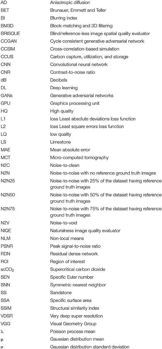
Keywords: image processing, micro-computed tomography, deep learning, denoising, image enhancement, digital rock physics, carbon capture utilization and storage (CCUS), enhanced oil recovery
Citation: Tawfik MS, Adishesha AS, Hsi Y, Purswani P, Johns RT, Shokouhi P, Huang X and Karpyn ZT (2022) Comparative Study of Traditional and Deep-Learning Denoising Approaches for Image-Based Petrophysical Characterization of Porous Media. Front. Water 3:800369. doi: 10.3389/frwa.2021.800369
Received: 23 October 2021; Accepted: 10 December 2021;
Published: 25 January 2022.
Edited by:
James E. McClure, Virginia Tech, United StatesReviewed by:
Tim Scheibe, Pacific Northwest National Laboratory (DOE), United StatesXiaofan Yang, Beijing Normal University, China
Copyright © 2022 Tawfik, Adishesha, Hsi, Purswani, Johns, Shokouhi, Huang and Karpyn. This is an open-access article distributed under the terms of the Creative Commons Attribution License (CC BY). The use, distribution or reproduction in other forums is permitted, provided the original author(s) and the copyright owner(s) are credited and that the original publication in this journal is cited, in accordance with accepted academic practice. No use, distribution or reproduction is permitted which does not comply with these terms.
*Correspondence: Miral S. Tawfik, mtawfik@alumni.psu.edu