


Political actors (countries, advocacy organizations, individual citizens) often interact spatially, and depend on each other through spatial relations. This holds in both monadic and dyadic phenomena. In international relations for example, spatial proximity affects interstate trade and war. Countries sharing borders are more likely to establish economic ties than countries farther apart (Beck et al., Reference Beck, Gleditsch and Beardsley2006; Allee and Scalera, Reference Allee and Scalera2012), whereas close spatial proximity also heightens the likelihood of territorial disputes (Mitchell and Trumbore, Reference Mitchell and Trumbore2014; Schultz, Reference Schultz2015). Spatial relations also play an important role in shaping the behavior of subnational actors. In the literature on civil conflict, interactions among actors like insurgent organizations, local governments, and civilian are critically shaped by their geographic territory, strongholds, and the hot-spots of conflict zones (Stephenne et al., Reference Stephenne, Burnley and Ehrlich2009).
Space regulates many aspects of political actors’ interactions. In several areas of political science, researchers have made substantial progress when it comes to the analysis of spatial dependence among fixed geographic units (e.g., Forsberg, Reference Forsberg2008; Seljan and Weller, Reference Seljan and Weller2011; Neumayer et al., Reference Neumayer, Plumper and Epifanio2014). However, despite applications that involve the study of actors with geographic information attached, we do not yet have a road map regarding how to analyze spatial dependence among actors that move. Examples of moving actors that are common in political research include militarized organizations in subnational conflict (Fjelde and Nilsson, Reference Fjelde and Nilsson2012), social media users (Larson et al., Reference Larson, Nagler, Ronen and Tucker2019), and social movement organizers (Cho et al., Reference Cho, Gimpel and Shaw2012). The central challenge in applying methods that are commonly used with static actors to the context of moving actors is the presence of multiple spatial observations for each actor. Furthermore, in dyadic moving actor data, locations are not observed independently for individual actors. Rather, locations often reflect the places in which dyadic interactions occurred (e.g., in subnational conflict data).
We propose a simple data-driven method to account for spatial patterns in dyadic interactions between moving actors. We develop an algorithm that uses the spatiotemporal histories of dyadic interactions to project where actors are likely to interact in the future, deriving projected actor locations (PALs), and use these PALs in models that predict dyadic interactions. Importantly, PALs represent predicted locations of moving actors’ interactions—not where they are headquartered or located in any other sense. This is an important point, because, aside from individuals, most moving political actors (e.g., militant organizations, advocacy groups, governments) can occupy more than one location at any given time. We offer three contributions to the existing literature. First, we make a substantive case that location information can and should be used to model dyadic interaction among moving actors in the same way as it is used to model interactions between actors in fixed locations. Second, we offer a methodology for integrating location history into location prediction. Third, we introduce the concept of using one dyadic actor's location history to help predict the other actor's location.
1. Accounting for interaction and movement in spatial dependence
Past work on conflict has recognized the importance of geographic components in both international and intrastate applications. However, as far as we can tell, with the exception of Beardsley et al. (Reference Beardsley, Gleditsch and Lo2015), geographic attributes of actors have been assumed to be fixed. In Beardsley et al. (Reference Beardsley, Gleditsch and Lo2015), the locations of subnational conflicts are studied as outcomes. Fixed location, of course, is a reasonable assumption in the interstate conflict literature. However, in subnational studies in which, e.g., rebel groups, are included among the actors many actors have no fixed geographic locations.
We propose a methodology for predicting locations in which actors are likely to interact in the future based on dyadic interactions. The core of the methodology we propose is a temporal smoothing function that integrates focal's (i.e., the actor being predicted) and alter's (i.e., the focal actor's opponent) spatial histories to produce a prediction of a future location of interactions. Our methodology represents a special case of exponential smoothing in time series (De Livera et al., Reference De Livera, Hyndman and Snyder2011).
In the most complex form of the PALs accounts for four aspects of location histories in the prediction of future interaction locations. First, we incorporate the average location of the focal actor's past history, whereby more recent interactions are weighted more heavily in the average. This reflects the expectation that actors’ locations are autocorrelated. Second, we incorporate the average locations of the interactions in which the focal actor's alters have engaged, again weighting recent interactions more heavily. This reflects the expectation that actors are likely to engage in places that their partners have recently been engaged. Third, to incorporate both the focal and alters’ histories, we set the location projection equal to a weighted average of the focal and alters’ location averages. Fourth, in making the projection, we let the relative weight of focal's and alters’ averages depend on the number of events going into each of the respective averages. This reflects the expectation that the predictive contribution of a location average will increase with the number of events incorporated into that average.
In the functions presented below, four parameters are included to project dynamic locations from dyadic event locations. The parameter α ≥ 0 controls the degree to which the contribution of a past event where the focal actor was engaged decays over time. The larger the value of α, the lower the weight placed on older events in projecting the locations of future events. The parameter β ≥ 0 controls the time decay of alters’ location histories. The larger the value of β, the lower the weight placed on older events in projecting the locations of future events. The parameter γ tunes the relative influence of a focal actor's locations relative to alter's locations. The higher the value of γ, the greater the weight placed on alters’ location averages. The last parameter we introduce, η, controls the degree to which the relative weight of focal and alter locations depends upon the number of events included in their histories. The larger the value of η, the greater the degree to which the relative influence of focal and alter histories depends on the relative number of events incorporated into their averages. The PALs algorithm is currently specified to weight actors according to the number of previous records that involve the respective actor. However, in the future this could be extended to account for other features of an actor, such as the variation in the locations in which they previously interacted. The functional forms according to which location histories are smoothed and combined to produce predicted actor location at time t, denoted $g_i^{( t) }$ , which are inspired by common functional forms used in exponential smoothing for time series forecasts (see, e.g., Equation 3 in Chatfield et al. (Reference Chatfield, Koehler, Ord and Snyder2001)), are given by,

where the function a(e) returns the age of event e, g(e) returns the location of event e, $E^{( t-) }_i$ is the set of events in which the focal actor was involved prior to time t, and $E^{( t-) }_k$
 is the set of events in which all of the actors with which the focal actor has been in conflict prior to time t have been involved. The resulting PAL is a predicted two-dimensional (i.e., latitude and longitude) coordinate for each individual actor, which can be interpreted as the location in which that actor is likely to engage in conflict in the near future. We have developed PALs to be directly applicable to any setting in which researchers have access to at least the timing and locations of dyadic interactions. However, the algorithm could be extended to account for other information on actors, events, and/or times. For example, a measure of event size and/or intensity could be incorporated into the weights of events. Such extensions would be valuable future methodological contributions.
We estimate the parameter values by minimizing the sum of the distances between projected and observed locations. Locations are represented in terms of latitude and longitude pairs. We consider two forms of the temporal smoothing function. In the full/four-parameter version, we estimate all of the parameters we have described above. The second version is a one-parameter model that uses only the focal actor's history. When we fix π = 0 (by, e.g., fixing γ = −∞), the influence of alter's history drops out of the function, making the function effectively monadic, and the only parameter that matters is α. We compare these two functions in order to analyze the predictive contribution of incorporating alters’ location histories into the projections.
2. Modeling sub-national conflict in Nigeria
Dorff and Gallop (Reference Dorff, Gallop and Minhas2020) model dyadic conflict between armed groups in the Nigerian civil conflict on an annual basis, for the years 2000–2016. The dyadic outcome variable is an indicator of whether or not two groups were in conflict in the respective year, for each year and each pair of groups. This study is innovative along two dimensions that are relevant to our analysis. First, the modeling approach used in the original paper, a recently-developed latent factor network model termed AMEN (Minhas et al., Reference Minhas, Hoff and Ward2019), is cutting-edge, which means that our contributions will be evaluated in the context of a sophisticated analytical framework. The model includes a probit-form regression equation that incorporates covariates, along with a set of actor-level latent variables that model network structure. Second, Dorff and Gallop (Reference Dorff, Gallop and Minhas2020) focus specifically on the out-of-sample predictive performance of the models they study, which offers a natural way for us to evaluate our contributions in the context of the original model. Using data from previous time points, we derive PALs for each group in each year. We expect that groups that are projected to be closer will be more likely to be in conflict than groups that are far apart.
To estimate parameters, we minimize the sum of the Haversine distances (i.e., arc distances on the sphere (Curley et al., Reference Curley, Manne and Veit2020) between predicted and observed event locations). The estimation of parameter values that are used for projecting the location at time t is obtained using a hill-climbing algorithm applied to event data from the times preceding t. We train this parameter optimization algorithm by using conflict events in Nigeria from the ACLED dataset (The Armed Conflict Location & Event Data) that Dorff and Gallop (Reference Dorff, Gallop and Minhas2020) use and the subset of armed groups used in their analysis. They focus on armed groups that are engaged in battles for at least 5 years during the 2000–2016 period, which results in a total of 37 armed groups. Since the unit of analysis is at the yearly level, we predict dyadic actor location at the year t by using the parameter(s) estimated in the previous years.
In order to accurately propagate the uncertainty in PALs through the parameter estimates in the models in which they are used, we use a bootstrap approach to generating a distribution of PALs. To generate a draw from the distribution of PALs, we take a full random sample with replacement of events over the full event dataset, and then re-run our PAL estimation procedure. This method of assessing uncertainty is special case of nonparametric bootstrap prediction (Fushiki et al., Reference Fushiki, Komaki and Aihara2005). We take a multiple imputation approach to using bootstrap samples of PALs to reflect uncertainty in model estimates. We treat each bootstrap sample as a random imputation within a multiple imputation framework. Bootstrap methods represent an alternative to the commonly-used parametric distributions for forming random imputations (Andridge and Little, Reference Andridge and Little2010). We use ten imputed samples of PALs in our application below, which is on par with the 5–20 imputation draws commonly observed in the literature (Rezvan et al., Reference Rezvan, Lee and Simpson2015). We run the statistical model ten times, one with each bootstrap prediction of PALs, and combine the results using Rubin's Rules for multiple imputation (Schafer and KOlsen, Reference Schafer and KOlsen1998). Since we use Bayesian Inference with AMEN, we treat the posterior means and standard deviations as analogous to the parameter estimates and standard errors, respectively.
Figure 1 shows the results of the parameter estimation for both the full four-parameter model and the α-only model. There are three points to take away from these results. First, the temporal decay parameter for the focal actor (α) is generally estimated to be much larger than the decay parameter for the alters’ locations (β), meaning that, to the degree that opponents’ past locations contribute at all to the prediction of focal's future location, the contribution of past opponents’ locations decays much more slowly. Relatively speaking, the focal actor's most recent locations are much more informative than past locations. Once transformed back onto the unit scale, the α values in all but the first couple of years are estimated to be around 0.9. This value corresponds to a significant decay in the weight of an event over time in predicting an actor's location. For example, an event that is two years old is weighted at 0.53 the rate at which events that are one year old are weighted. This weight drops to 0.29 for events that are four years old. Second, the consistent negative signs of γ and η indicate, respectively, (1) that opponents’ locations are generally not weighted very heavily in projecting future locations, and (2) that the influence of opponents’ locations decays quickly as the focal actor accumulates a more frequent history of interaction. Third, the substantial variation in parameter estimates across bootstrap samples, as indicated by the gray regions, demonstrates the importance of accounting for uncertainty in the PALs.
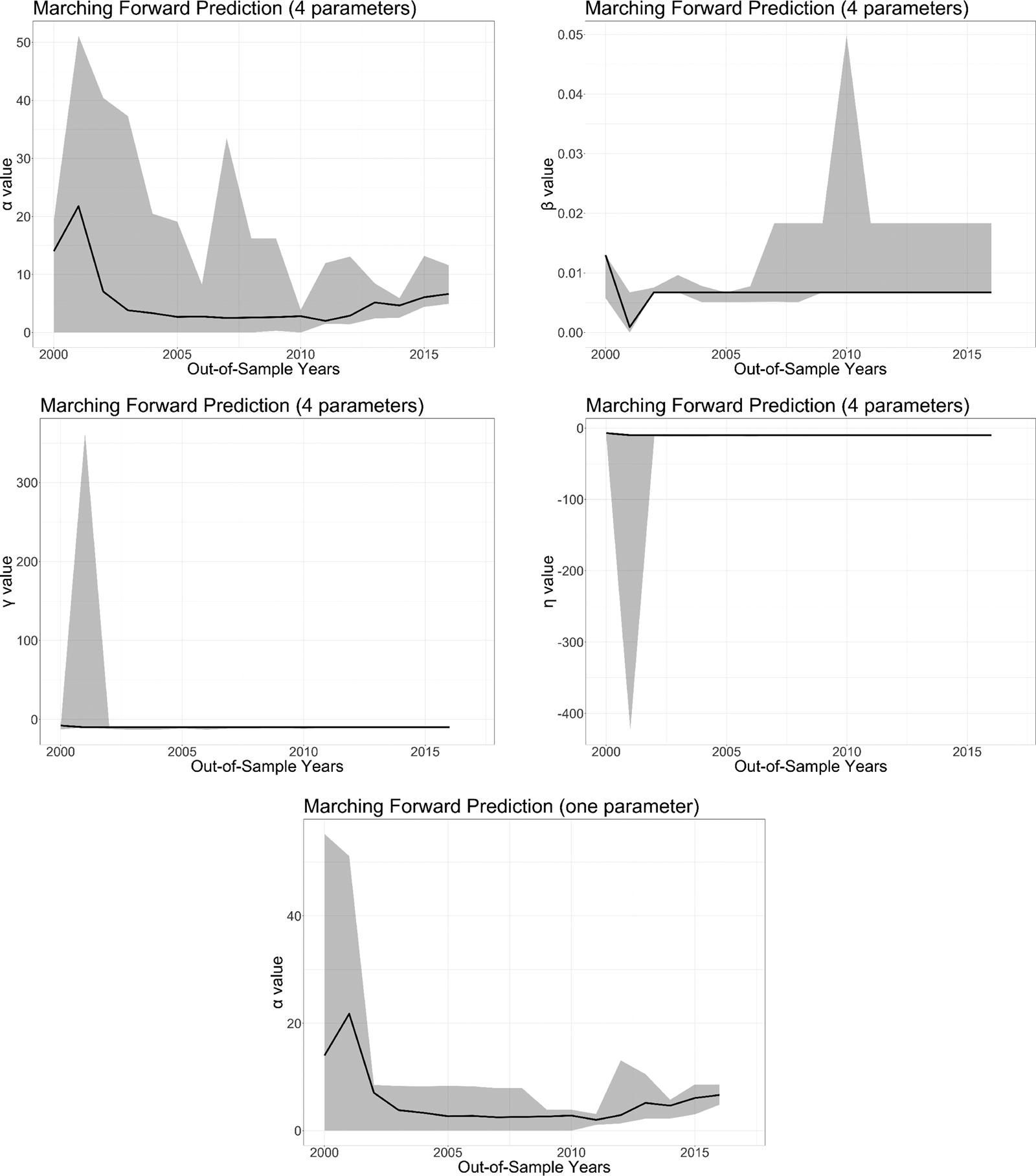
Figure 1. Parameter estimates by year. Parameters for the given year are estimated using all values observed before the respective year. The solid black line gives the values estimated on the complete observed data, and the light gray region depicts the range of values calculated under the ten bootstrap samples.
To evaluate the predictive performance, we use a marching-forward prediction that uses dyadic location history in the past years to predict movements in the current year. To compare parameter constraints, we calculate the average Haversine distances between the observed locations and the PALs. In Figure 2, we present the forecasting performance results. We see that there is no clear improvement in performance from adding the alter information. Still, since the differences between the two models are minimal, in the application below we will specify models with two different types of predicted distance variables: one in which α, the time decay of the focal actor's event history, is the only active parameter, and the other one with all parameters active. We include both forms of location prediction to evaluate whether results from the extension are robust to either specification. In future applications with the PAL methodology, researchers could use a predictive experiment, such as the one we present in Figure 2 to select between the focal-only and full approaches. In our case, one method does not perform clearly better than the other.
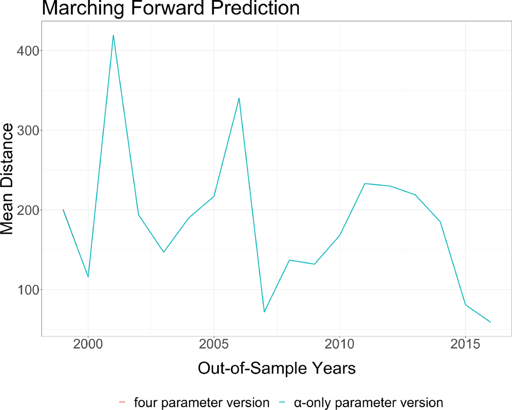
Figure 2. Mean haversine distance between forecast and observed locations.
Since the potential contribution of our PALs to the performance of models in which they are used is tied to their performance in predicting future locations, we conduct some additional investigation into the predictive accuracy of the PALs. In Figure 3 we present results from two accuracy checks. In the first plot we map observed and predicted event locations on the map of Nigeria, and draw an edge from the predicted to the observed location. Most of the ties span short distances, indicating the relative accuracy of PALs. However, in some years, we do observe edges that span substantial distances. We do not see any patterns in terms of the types of groups, or time periods, for which PALs are more or less accurate. What we present in the second plot is more informative regarding the overall performance of the PALs in predicting where future events will occur. The plot includes two boxplots for each year. In the first/red boxplot, we depict the distributions of distances between the locations of the events that occurred in the respective year. If the PALs are improving our predictions of where events will occur, the distances between observed event locations and predicted event locations should be, on average, smaller than the distances between randomly selected events in the same year. The second/gray boxplot depicts the distribution of distances between observed events and their predicted locations. We see that the distances between predicted and observed locations are smaller than the distances between observed events in all but two years, indicating that the predictions are close, in relative terms, to the observed locations. The effectiveness of PALs in predicting conflict locations is dependent on the degree of memory, or autocorrelation, in the spatial locations in which groups engage in conflict. In both 2001 and 2006, which are the worst-performing years in terms of predicting conflict locations, groups get involved in conflicts in regions of the country where they have not previously operated.
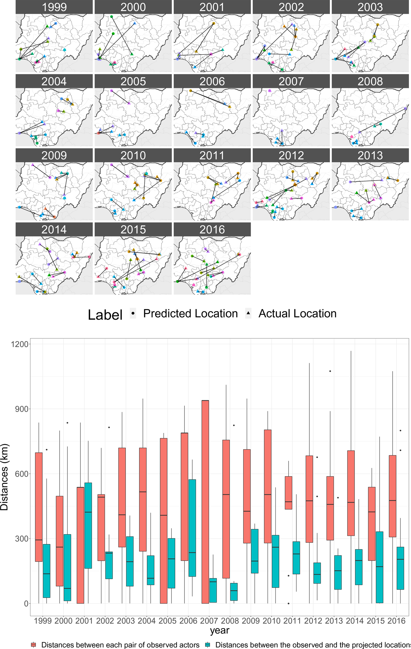
Figure 3. Comparison of PALs and observed locations. In the top plot, edges are drawn from predicted to observed event locations. In the bottom plot, we compare differences between observed event locations to differences between predicted and observed event locations.
To illustrate the interplay in the PALs between observed event locations, projections, and time, we focus on an example from subnational conflict in Nigeria, focusing specifically on the Christian Militia. We look at the Christian Militia since they have an extensive history of events in our data, and exhibit substantial geographic variability in event locations. This example is presented in Figure 4. We depict projected and observed event locations for the years 2001 through 2016. We note two illustrative observations from this example. First, up through 2009, most of the conflict events in which the Christian Militia is involved occur in the northern half of the country. In 2010, they are involved in a conflict event in the southern half of the country. We can see the effect of this southern event in the 2011 projections, in which they shift down toward the center of the country. Second, the uncertainty in the PALs, as represented by the distribution of projections, is greater earlier on in the time series, where the PALs are trained on less data, than later on in the time series, where projections are informed by more data.
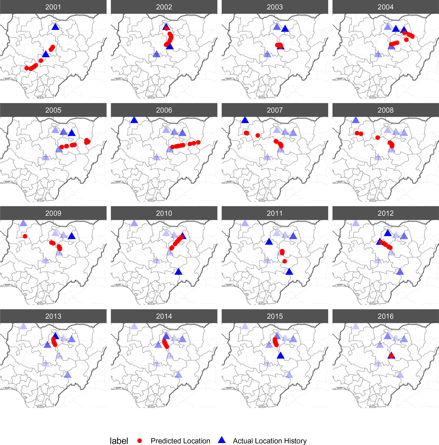
Figure 4. Example history of projected and observed event locations for the Christian Militia. Projections plotted are from the full four-parameter function, but results are extremely similar to the one-parameter specification. There are ten projected locations in each year, based on the bootstrap samples. The (blue) shading of observed events becomes lighter with the age of an event.
2.1. Replication and extension of Dorff and Gallop (Reference Dorff, Gallop and Minhas2020)
We ran the AMEN models for 10,000,000 MCMC iterations, whereas Dorff and Gallop (Reference Dorff, Gallop and Minhas2020) ran the original model for 50,000 iterations. We did this due to minor evidence of non-convergence in the original models with 50,000 iterations (Gill, Reference Gill2008). The traceplots all appear in the Appendix. In this section we present the original model with 50,000 iterations, the original model with 10,000,000 iterations, and models that include the distance between two groups’ PALs’ as a covariate—estimated with 10,000,000 iterations.
We consider two alternative specifications of PAL distance. First, we include a “linear” specification in which the Haversine distance between two groups’ PALs is included as a covariate. Second, we include a “logged/ln” specification in which the natural log of the Haversine distance between two groups’ pals is included as a covariate. The log specification of (e.g., Werner, Reference Werner2000; Jungblut and Stoll, Reference Jungblut and Stoll2002) geographic distance is most common in the study of interstate dispute, but we look at both linear and log since distances in intrastate conflict are on a smaller scale, and are more constrained.
We present the results of our replication analysis in Table 1. The first and second columns include the results of the original specifications with 10,000,000 and 50,000 iterations, respectively. The extended model, including the PAL distance variables, are included in columns 3–6. We see that the geographic distance variable, based on both the linear and log specifications, has a statistically significant negative effect on the likelihood of conflict. As the distance between two groups’ projected locations increases, the likelihood of conflict between them decreases.
Table 1. Dorff and Gallop (Reference Dorff, Gallop and Minhas2020) replication results
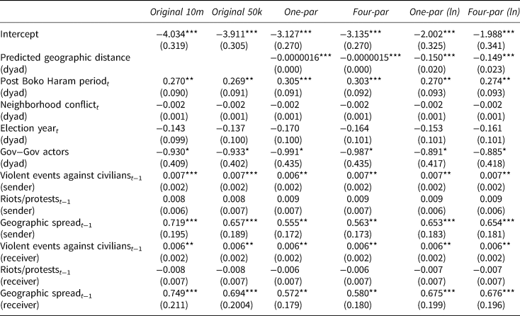
Note: AMEN results. Posterior mean coefficients reported with posterior standard deviations, calculated over ten bootstrap imputations of PALs, in parentheses. *p < 0.05; **p < 0.01; ***p < 0.001.
In Figure 5 we present visual interpretations of the effect of distance on the probability of conflict. Given average values of the other variables in the model, the probability of conflict goes from a value between 0.01 and 0.02 at very low projected distance (0–100 km), to values of 0.001 or less at projected distances of 500 km or more, representing a tenfold decrease in the likelihood of conflict. The log specification, which is more common in the literature on international conflict and provides a slightly better out-of-sample predictive fit in the current application, indicates that the probability of conflict decreases quite quickly with distance—dropping from approximately 0.01 to 0.001 within a span of 200 km. Considering that Nigeria is approximately 1000–1100 km across in both directions, this finding is substantively meaningful.
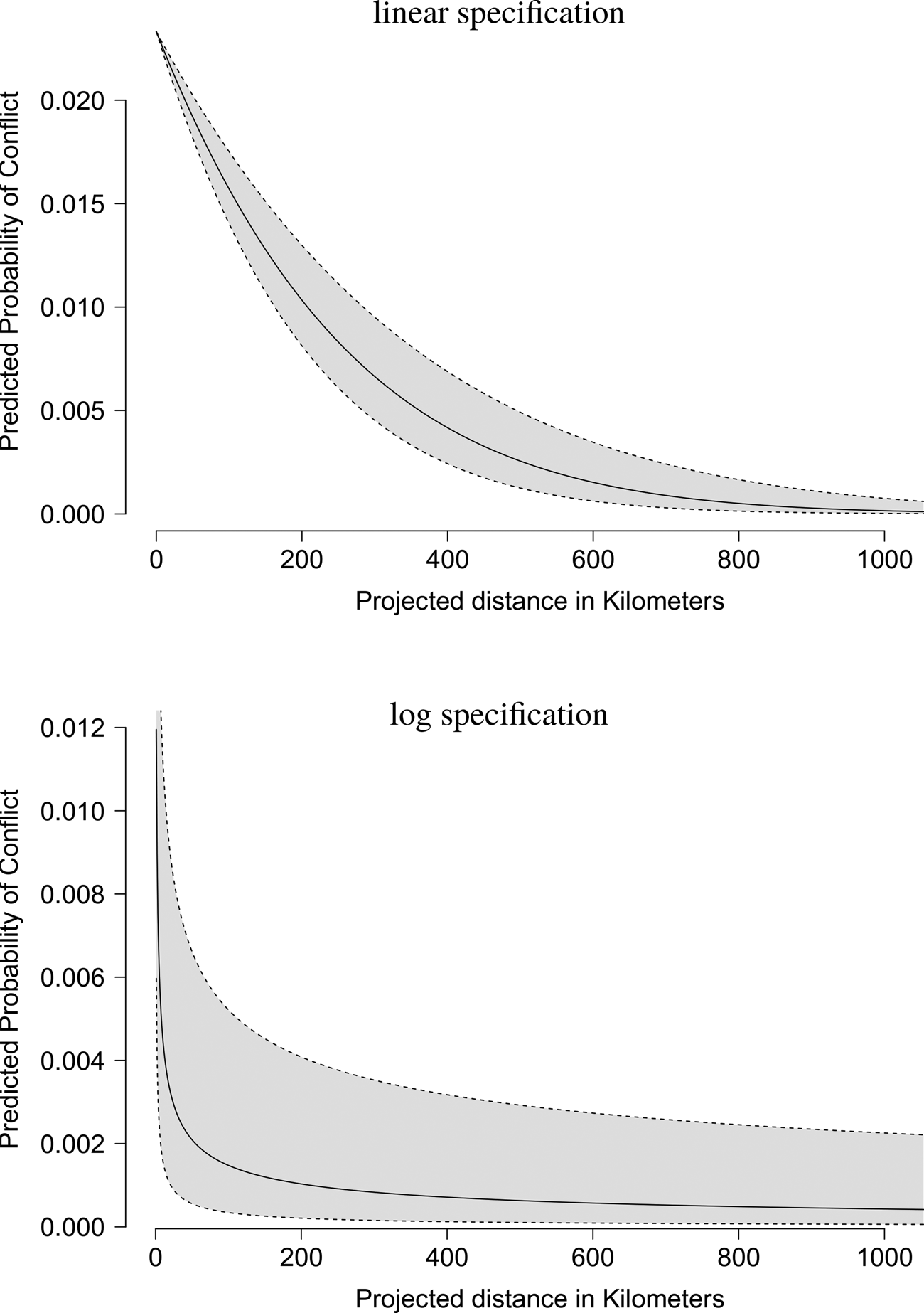
Figure 5. Predicted probability of conflict based on linear and natural log distance specifications. These plots are based on the four-parameter PALs, but are virtually equivalent to those using the one-parameter PALs.
When it comes to the other variables in the model, the signs and significance of estimates are unaffected by the addition of PALs to the models. However, the magnitudes of some of the coefficients shift significantly. Interestingly, though perhaps not surprisingly, the largest shifts in magnitude occur in the estimates of the variables associated with the geographic spread of conflict.
We now turn to assessing the projected distance variable's contribution to out-of-sample fit of the model, as assessed in Dorff and Gallop (Reference Dorff, Gallop and Minhas2020). As we have done for the main results, we also reran the analysis conducted by Dorff and Gallop (Reference Dorff, Gallop and Minhas2020) with 10,000,000 iterations to assure comparability with our results. Predictive performance is assessed by splitting the data into 30 groups, and iteratively holding out, and then predicting, the dyadic conflict outcomes in each group. Figure 6 shows the replicated predictive performance assessments of the original and all four extended models. Receiver Operator Characteristics (ROC) curves examine trade-off between true-positive rates and false-positive rates while precision-recall (PR) curves assess trade-off between the proportion of predicted conflicts by a model and the proportion of predicted conflicts which actually occur. As conflict events are rare, the area under the PR curve provides a more accurate assessment of predictive performance compared to the area under the ROC curve (Cranmer and Desmarais, Reference Cranmer and Desmarais2017).
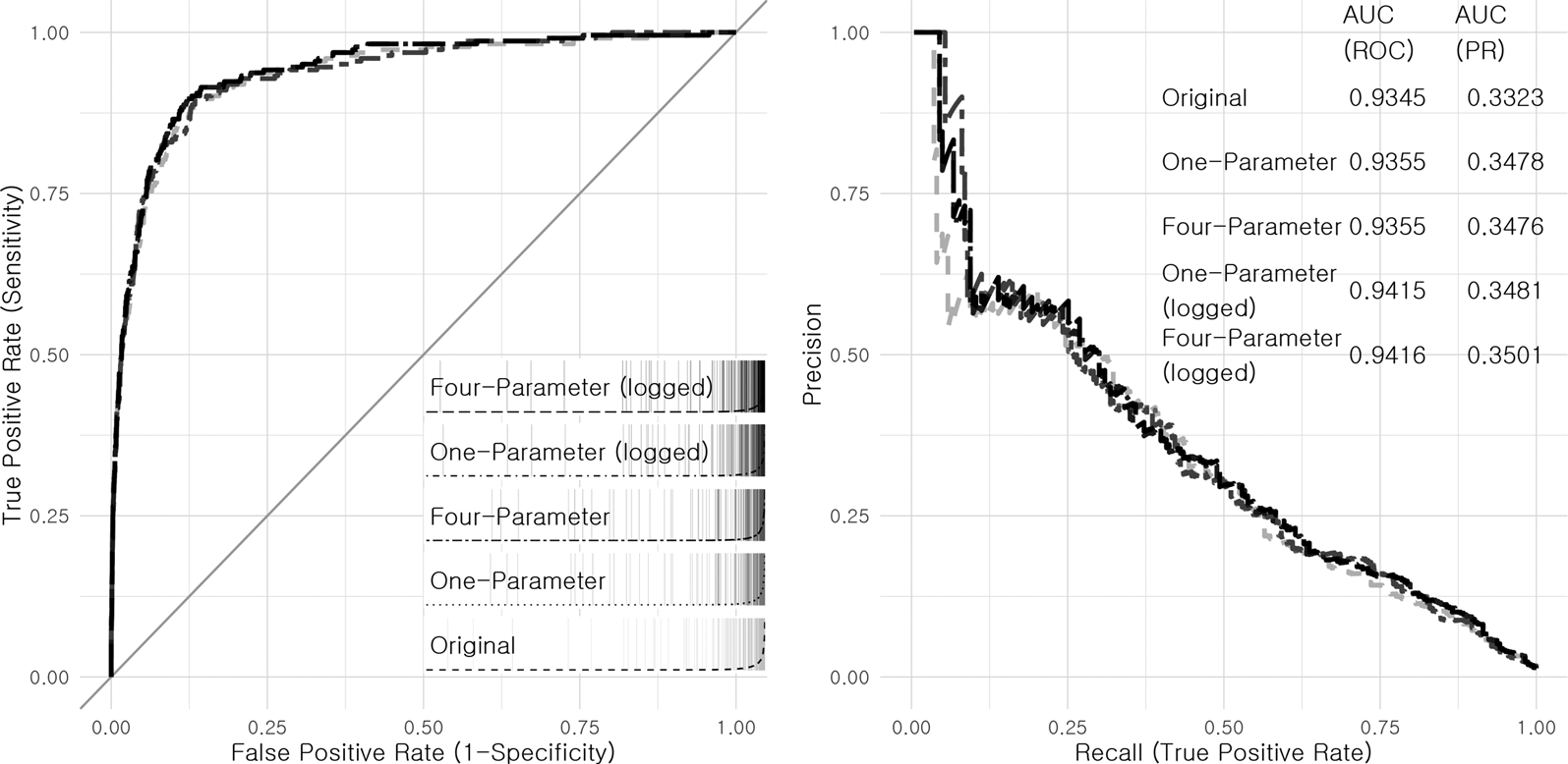
Figure 6. Out-of-sample predictive performance
Adding the predicted distance variable improves the predictive performance of the model in all four variants of the extended model. There is a slight increase in both the areas under the ROC and PR curves. One notable result is that the greatest improvements in fit result from the log specification, and the model that fits best out-of-sample includes the four-parameter PALs with the log specification. The predictive improvements are only modest—at the very least, we can be confident that adding the distance variables does not represent an instance of over-fitting the data. However, combined with the statistically and substantively significant in-sample results, the predictive improvements further point to the value in accounting for the spatial dynamics of moving actors.
Conclusion
Spatial dynamics are tightly linked with conflict dynamics at both the international and subnational levels. This is true of conflict and many other political phenomena. With the growing availability of fine-grained spatial data (e.g., event data, social media traces) that covers moving actors, modeling the spatial dynamics of political activity means accounting for movement in space. We provide a straightforward approach to projecting the locations in which moving actors are likely to interact in the future, using data on past dyadic events. We apply our approach to a replication and extension of an analysis of subnational conflict. The results indicate that geographic proximity, as measured through the projection of dynamic actor locations, plays an important role in explaining subnational conflict.
Supplementary material
The supplementary material for this article can be found at https://doi.org/10.1017/psrm.2022.6. To obtain replication material for this article, please visit https://doi.org/10.7910/DVN/NLWWPE


 Open access